Multiple Linear Regression in R: A Powerful Analysis Tool

Overview

Have you ever thought about how to analyze the relationship between multiple variables using R? If so, then this article is for you. After reading this article, you will be able to perform multiple linear regression in R.

Multiple linear regression is a popular statistical method to analyze the relationship involving multiple predictor (independent) variables with one response (dependent) variable. We can perform multiple linear regression in R or Python. In this article, we will show you how to perform multiple linear regression in R.

In this article, you will learn:

• What is multiple linear regression?

• What are the various assumptions of multiple linear regression?

• How to implement multiple linear regression in R?

• How to check the validity and accuracy of the regression model?

• How to use the model for prediction on new (unseen) data?

If you are ready to learn the fascinating topic then dive in!

What Is Multiple Linear Regression?

In multiple linear regression, we try to find the relationship between a response variable (dependent variable) with its predictor variables (independent variables). For simple linear regression, there is only one predictor but in multiple linear regression, there is always more than one predictor.

Let us try to understand multiple linear regression, with the help of a simple example. Suppose you are a business analyst who works for a company. Your job is to understand how the profit of each laptop (profit) depends on various factors: speed of the processor (processor), size of the screen (screen), life of the battery (battery), and rating of the customer (customer).

To do so, you need to collect a lot of data (say, 100 observations) on laptop models and their profits. If you decide to use multiple linear regression as a predictive model then you can express the response (profit of each laptop) as a function of predictors as,

$profit=b_0+b_1\times processor+b_2\times screen+b_3\times battery+b_4\times rating$

In the above equation, b0, b1, b3, and b4 are the coefficients that need to be evaluated from the data using multiple linear regression.

In a more generic form, we can express multiple linear regression as,

$y=b_0+b_1x_1+b_2x_2+b_3x_3+…..+b_nx_n$

Where,

y is the response (dependent) variable, x represents the predictor (independent) variables, and n is the total number of predictor (independent) variables.

Assumptions Of Multiple Linear Regression

We need to check several assumptions before performing multiple linear regression. Let us discuss them one by one briefly

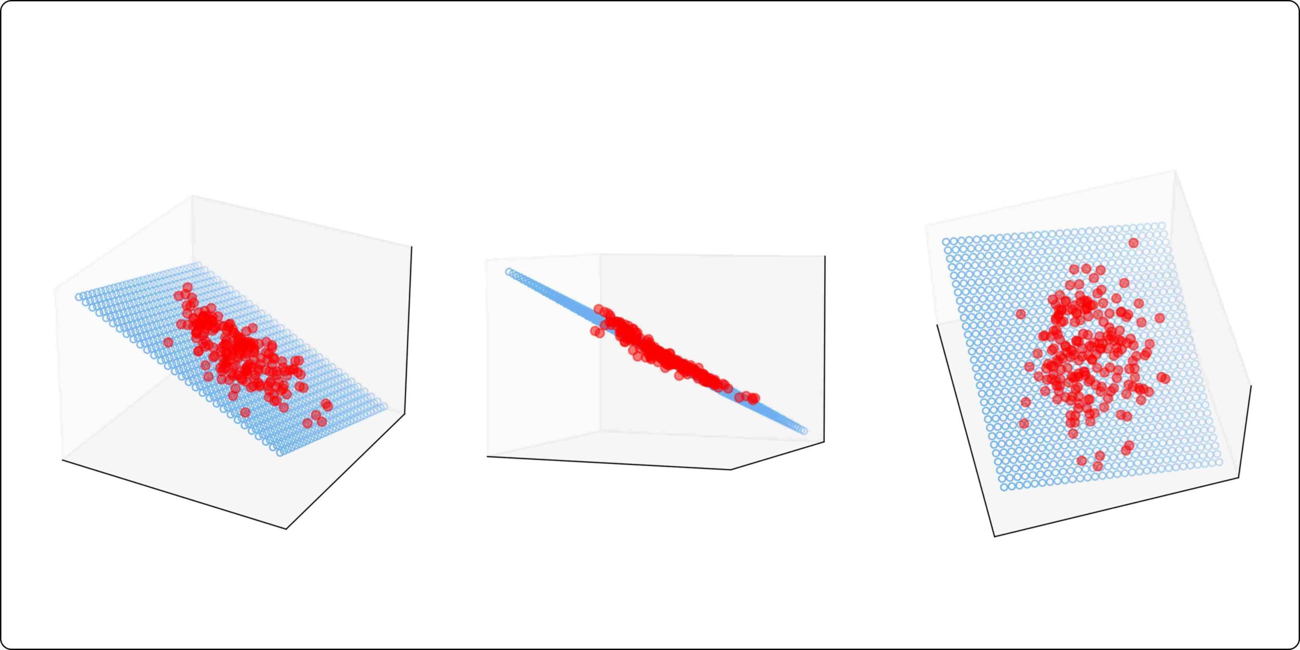
Linear Relationship

Multiple linear regression assumes a linear relationship between response and predictor variables. We can visually inspect the linear relationship with the help of a scatter plot.

No multicollinearity:

Predictor variables should not be highly correlated with each other. We can use a correlation matrix or variance inflation factors (VIF) to measure multicollinearity.

Independence:

The observations should be independent of each other. One of the popular methods to check the autocorrelation among residuals is the Durbin-Watson test.

Multivariate normality

The residuals should be normally distributed. There are various methods such as Q-Q plots, Shapiro-Wilk, or Kolmogorov-Smirnov for checking normality.

Homoscedasticity

The variance of the residuals should be constant across the values of the predictor variables. We can use the residual plots /Breusch-Pagan test to check heteroscedasticity.

How To Implement Multiple Linear Regression In R?

In this section, we will implement multiple linear regression in R to find relationships among the startup datasets. You can find the code and data in the following links: Code and Data

Understanding The Data

We have a dataset containing information on 50 startups. Each row of the table below shows the profit of a startup based on R&D Spend, Administration, Marketing Spend, and State. The aim is to implement multiple linear regression in R to model the relationship between the response variable (profit) and predictor variables (R&D Spend, Administration, Marketing Spend, and State).

The figure below shows a snapshot of the dataset (Figure 1).

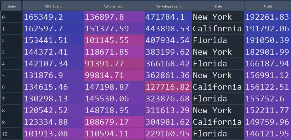
Figure 1: Snapshot of the startup dataset used for multiple linear regression

Install Libraries

Here, we will install caTools which is a collection of various utility functions in R. The caTools can be used for data splitting, generating indices, and sample size calculation in data science.

If you already have caTools installed, you can skip this step. Otherwise, run the following line once in your R environment.

install.packages('caTools')

Import Dataset

Next, we load the startup dataset into R using read.csv(). Make sure the file StartupData.csv is available in your current working directory.

dataset = read.csv('StartupData.csv')

Categorical Data Encoding

In categorical data encoding, categorical variables are transformed into numerical values so that they can be used for statistical analysis. There are various methods for categorical data encoding in R, such as Level encoding, One hot-encoding, and Frequency encoding.

The dataset we considered here has a categorical variable named “State” that can take values such as “New York”, “California” or “Florida”. The figure below shows a snapshot of the dataset (Figure 1).

Figure 1: Snapshot of the startup dataset used for multiple linear regression

The above code snippet uses the Level encoding method to convert categorical data into numerical values. As we can see in the table below (Figure 2), the categorical data (New York, California, and Florida) are replaced with numerical values (1, 2 and 3).

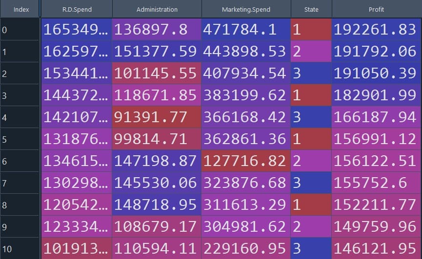
Figure 2: Dataset after categorical data encoding

dataset$State = factor(dataset$State, levels = c('New York', 'California', 'Florida'), labels = c(1, 2, 3))

Split the dataset into Train set and Test set

Here we used, caTools to split the dataset into training and testing sets. We here considered a SplitRatio=0.75 to split the data.

In simple terms, we train the model on 75% of the data and keep 25% aside to evaluate how well the model performs on unseen rows.

library(caTools)
set.seed(123)
split = sample.split(dataset$Profit, SplitRatio = 0.75)
training_set = subset(dataset, split == TRUE)
test_set = subset(dataset, split == FALSE)

Fitting Multiple Linear Regression to the Training set

Let us fit a multiple linear regression model in R using the lm function. In the lm function, profit is defined as the response variable, and the rest of the variables in the dataset are defined as predictor variables.

The formula Profit ~ . means: “predict Profit using all remaining columns in the dataset as predictors.”

regressor = lm(formula = Profit ~ ., data = training_set)

Predicting the Test set results

Let us predict the model performance on the test dataset.

This will generate predicted profit values (y_pred) for the rows in test_set.

y_pred = predict(regressor, newdata = test_set)

Visualize Model Prediction

To make the results easier to interpret, we can place the predicted profits next to the actual profits and compare them side-by-side.

%%R
y_test=test_set$Profit
comparison <- cbind(y_pred, y_test)
print(comparison)

• The table on the right-hand side compares the predicted value of the response variable using multiple linear regression with respect to the observed value.

• We can see from the figure that the value predicted by multiple linear regression is quite close to the original value.

• In the next step we will evaluate the performance of the multiple linear regression model using various metrics.

-

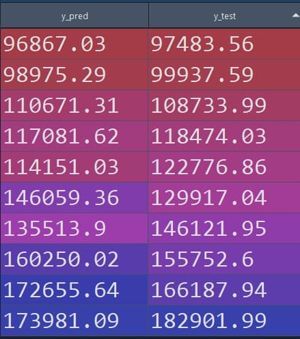
Figure 3: Predicted vs observed values (tabular comparison)

Model Evaluation and Validation

We can evaluate the performances of the multiple linear regression model with the help of various matrices such as mean squared error (MSE), root mean squared error (RMSE), and R-squared. Let us evaluate those :

Each metric gives a slightly different view of model quality:

• MSE/RMSE: how far predictions are from the actual profit values (lower is better)

• R-squared/Adjusted R-squared: how much variance in profit is explained by the predictors (higher is better)

Compute Mean Squared Error (MSE)

MSE measures the average squared difference between predicted and actual values.

mse <- mean((y_pred - y_test)^2)
print(paste("Mean Squared Error (MSE):", mse))

Mean Squared Error (MSE): 59614884.0721883

Compute Root Mean Squared Error (RMSE)

RMSE is simply the square root of MSE, so it is in the same unit as the target variable (profit), which is often easier to interpret.

rmse <- sqrt(mse)
print(paste("Root Mean Squared Error (RMSE):", rmse))

Root Mean Squared Error (RMSE): 7721.0675474437

Compute R-squared

R-squared tells you how much of the variation in the response variable is explained by the predictors.

rsquared <- 1 - sum((y_test - y_pred)^2) / sum((y_test - mean(y_test))^2)
cat("R-squared:", rsquared, "\n")

R-squared: 0.9210359

Compute Adjusted R-squared

Adjusted R-squared adds a penalty for adding too many predictors, so it’s often a better metric when comparing models with different numbers of features.

n <- nrow(test_set)
p <- length(coefficients(regressor)) - 1
adjusted_rsquared <- 1 - ((1 - rsquared) * (n - 1)) / (n - p - 1)
cat("Adjusted R-squared:", adjusted_rsquared, "\n")

Adjusted R-squared: 0.8223309

Conclusion

This article starts with the basics of multiple linear regression and understanding the mathematics of it that relates a response variable with multiple predictor variables. We also discussed various assumptions that need to be met before applying multiple linear regression in R to find relationships among variables.

In this article, we implemented multiple linear regression in R to find the relationship between the profit of a startup based on R&D spending, administration, marketing spending, and state. Applying multiple linear regression in R is quite straightforward due to its user-friendly interface and extensive statistical libraries.

The performance of the model is further evaluated using various matrices such as mean squared error, root mean squared error, and adjusted R-squared. By analyzing the performance metrics, one can get a comprehensive understanding of how multiple linear regression captures the relationship between a response variable and multiple predictor variables.

Multiple linear regression is a powerful method for finding relationships between a response variable and multiple predictor variables. We can apply multiple linear regression in various sectors such as finances, economics, marketing, healthcare, education, and environmental science.

Frequently Asked Questions

What is one reason for performing multiple regression analysis?

Multiple linear regression helps to determine how several independent variables collectively influence a dependent variable. This helps a clear and comprehensive understanding of the factors affecting the outcome.

What is the advantage of using a multiple regression design?

Multiple linear regression allows us to analyze the impact of multiple independent variables simultaneously. This helps to make more accurate predictions and a deeper understanding of the relationships between variables.

References

Multiple Linear Regression In R

Multiple Linear Regression In Python

Multiple Linear Regression: Quick Guide

Simple Linear Regression In R