What Is VGG Net?
Do you know that the VGGNet developed by the Visual Geometry Group at the University of Oxford is one of the most groundbreaking convolutional neural networks? The architecture is known for its simplicity, involving 3×3 convolutional filters stacked on the top of each other. The network was developed to address the limitations of previous models like AlexNet by using smaller convolutional filters.
There are two main variants of VGGNet: VGG-16 and VGG-19. They consist of 16 and 19 layers, respectively. The depth of VGGNet combined with the use of smaller convolutional filters was a game-changer, pushing the boundaries of image classification accuracy.
VGGNet excels for various tasks and datasets beyond ImageNet benchmarks and is one of the most widely used image recognition architectures. Let us dive deep into this visually intuitive network and uncover its secrets!
VGG-16 Architecture
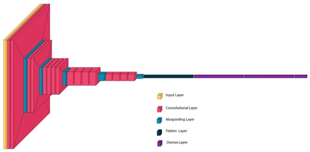
VGG16 is one of the popular architectures of VGGNet, as proposed by A. Zisserman and K. Simonyan from the University of Oxford. It has 16 layers: 13 convolutional layers, three fully connected layers, and five max-pooling layers. Figure 1 below shows a pictorial representation of VGG16 architecture. The model secured second place in the image classification task, achieving a top-5 test accuracy of 92.7% on the ImageNet dataset.
VGG16 replaced large kernel-sized filters of the AlexNet model with several 3×3 kernel-sized filters in succession. By doing so, VGG16 achieved significant improvements over AlexNet. Moreover, using small 3×3 convolution filters throughout the network makes the architecture uniform and simple.
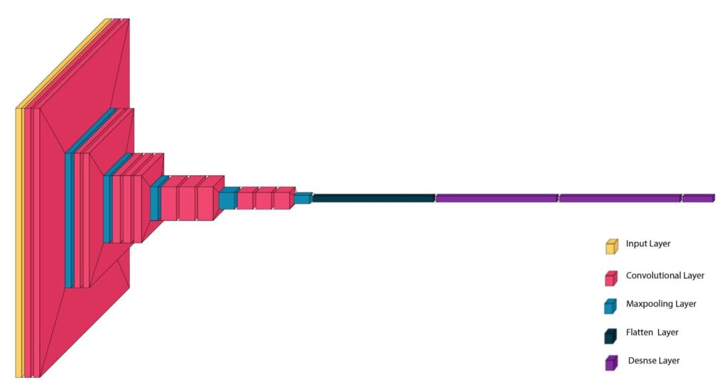 Figure 1: Pictorial representation of VGG16 architecture
The following are the key components of VGG16 architecture. You can also find the details of the various components of VGG16 in Figure 2 and Table 1 below.
Input Size
The input size of an image in VGG16 is 224×224 pixels with three color channels (RGB).
Convolutional Layers
VGG16 has 13 convolutional layers. The convolutional layers use small 3×3 filters, which are the smallest size and are capable of capturing spatial hierarchies like edges and textures. These layers are organized into blocks, with each block being followed by a max-pooling layer to reduce spatial dimensions and computational load.
The convolutional layers apply filters to the input image and perform dot products between the filter weights and local input regions, creating feature maps that emphasize different aspects of the image.
ReLU Activation Function
VGG16 uses the Rectified Linear Unit (ReLU) activation function after each convolutional layer. This helps to introduce non-linearity and helps the network to learn complex patterns.
Max-Pooling Layers
VGGNet uses several max-pooling layers with a 2×2 filter and a stride of 2. These layers help reduce the spatial dimension of the data, reducing the computational load. It also helps to control overfitting.
Fully Connected Layers
The network ends with three fully connected layers. Among the three layers, the first two layers have 4096 channels each, while the third has 1000 channels, 1 for each class. These layers help to convert 2D feature maps into a 1D feature vector. They act as a classifier on the top of the extracted features.
Softmax Output Layer
The final layer of the network is a SoftMax output layer. The output from this layer is the probability distribution over the classes, which is ideal for classification tasks.
Uniform Architecture
VGG16 uses small 3×3 convolution filters throughout the network, making the architecture uniform and simple. This helps VGG16 to capture fine details in the images.
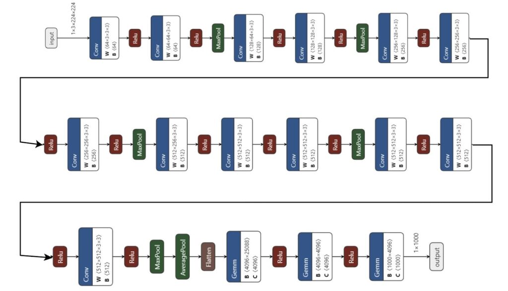
Figure 2: Visualizing VGG-16 layers, convolutions, and max-pooling
Table 1: Details of various layers, their output shape, and number of parameters of VGG-16
| Layer | Type | Output Shape | Number of Parameters |
|---|---|---|---|
| Input | - | (224, 224, 3) | 0 |
| Conv1_1 | Convolutional | (224, 224, 64) | 1,792 |
| Conv1_2 | Convolutional | (224, 224, 64) | 36,928 |
| MaxPooling1 | MaxPooling | (112, 112, 64) | 0 |
| Conv2_1 | Convolutional | (112, 112, 128) | 73,856 |
| Conv2_2 | Convolutional | (112, 112, 128) | 147,584 |
| MaxPooling2 | MaxPooling | (56, 56, 128) | 0 |
| Conv3_1 | Convolutional | (56, 56, 256) | 295,168 |
| Conv3_2 | Convolutional | (56, 56, 256) | 590,080 |
| Conv3_3 | Convolutional | (56, 56, 256) | 590,080 |
| MaxPooling3 | MaxPooling | (28, 28, 256) | 0 |
| Conv4_1 | Convolutional | (28, 28, 512) | 1,180,160 |
| Conv4_2 | Convolutional | (28, 28, 512) | 2,359,808 |
| Conv4_3 | Convolutional | (28, 28, 512) | 2,359,808 |
| MaxPooling4 | MaxPooling | (14, 14, 512) | 0 |
| Conv5_1 | Convolutional | (14, 14, 512) | 2,359,808 |
| Conv5_2 | Convolutional | (14, 14, 512) | 2,359,808 |
| Conv5_3 | Convolutional | (14, 14, 512) | 2,359,808 |
| MaxPooling5 | MaxPooling | (7, 7, 512) | 0 |
| Flatten | - | (7 * 7 * 512) | 0 |
| Fully Connected1 | Dense | -4096 | 102,764,544 |
| Fully Connected2 | Dense | -4096 | 16,781,312 |
| Output | Dense (Softmax) | -1000 | 4,097,000 |
VGG-19 Architecture
VGG19 is another popular variant of the VGGNet, developed by the Visual Geometry Group at the University of Oxford. The network is very similar to VGG16 but with a deeper architecture, comprising 19 layers: 16 convolutional layers, three fully connected layers, and five max-pooling layers. The figure below (Figure 3) shows a pictorial representation of VGG19 architecture.

Figure 3: Pictorial representation of VGG19 architecture
You can also find the details of the various components of VGG19 in the figure and table below.
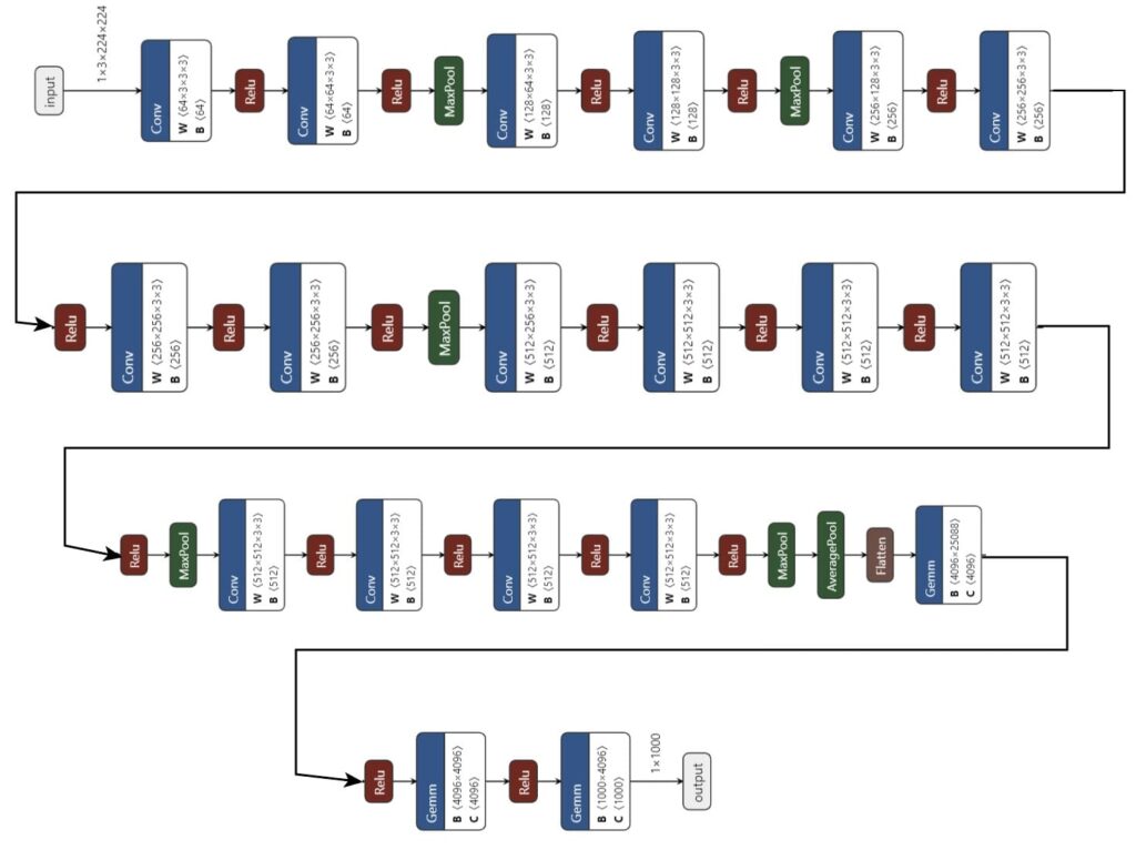
Figure 4: Visualizing VGG-19 layers, convolutions, and max-pooling
Table 2: Details of various layers, their output shape, and number of parameters of VGG-19
| Layer | Type | Output Shape | Number of Parameters |
|---|---|---|---|
| Input | - | (224, 224, 3) | 0 |
| Conv1_1 | Convolutional | (224, 224, 64) | 1,792 |
| Conv1_2 | Convolutional | (224, 224, 64) | 36,928 |
| MaxPooling1 | MaxPooling | (112, 112, 64) | 0 |
| Conv2_1 | Convolutional | (112, 112, 128) | 73,856 |
| Conv2_2 | Convolutional | (112, 112, 128) | 147,584 |
| MaxPooling2 | MaxPooling | (56, 56, 128) | 0 |
| Conv3_1 | Convolutional | (56, 56, 256) | 295,168 |
| Conv3_2 | Convolutional | (56, 56, 256) | 590,080 |
| Conv3_3 | Convolutional | (56, 56, 256) | 590,080 |
| Conv3_4 | Convolutional | (56, 56, 256) | 590,080 |
| MaxPooling3 | MaxPooling | (28, 28, 256) | 0 |
| Conv4_1 | Convolutional | (28, 28, 512) | 1,180,160 |
| Conv4_2 | Convolutional | (28, 28, 512) | 2,359,808 |
| Conv4_3 | Convolutional | (28, 28, 512) | 2,359,808 |
| Conv4_4 | Convolutional | (28, 28, 512) | 2,359,808 |
| MaxPooling4 | MaxPooling | (14, 14, 512) | 0 |
| Conv5_1 | Convolutional | (14, 14, 512) | 2,359,808 |
| Conv5_2 | Convolutional | (14, 14, 512) | 2,359,808 |
| Conv5_3 | Convolutional | (14, 14, 512) | 2,359,808 |
| Conv5_4 | Convolutional | (14, 14, 512) | 2,359,808 |
| MaxPooling5 | MaxPooling | (7, 7, 512) | 0 |
| Flatten | - | (7 * 7 * 512) | 0 |
| Fully Connected1 | Dense | -4096 | 102,764,544 |
| Fully Connected2 | Dense | -4096 | 16,781,312 |
| Output | Dense (Softmax) | -1000 | 4,097,000 |
Performance Of The VGGNet
The performance of VGG16 in the ILSVRC-2012 and ILSVRC-2013 competitions was found to be superior to earlier models, such as AlexNet. Its performance was on par with GoogLeNet (the classification task winner), which had an error rate of 6.7%. For single-network performance, VGG16 also achieved remarkable results with an error rate of approximately 7.0%, surpassing GoogLeNet by around 0.9%.
VGG19 also achieved a top-5 error rate of around 7.3% in the ILSVRC-2014 competition. Although the result was higher than the 7% error rate of VGG 16, the deeper architecture of VGG19 allowed it to capture more complex features and improve classification accuracy.
Complexity and Challenges
Although the VGGNet is known for its simplicity and effectiveness, it also has several complexities and challenges.
High Computational Demand
The number of parameters in VGGNet is very high. For instance, the VGG-16 has over 138 million parameters, resulting in a model size of more than 500MB. Due to this, the VGGNet requires significant computational power and memory. The large size of VGGNet can be challenging to deploy for devices with limited storage and memory.
High computational demand also translates to higher energy consumption. This can be a concern for large-scale deployments and environmentally-conscious applications.
Training Time
The training time of VGGNet can often be time-consuming. For instance, training VGG-16 on large datasets like ImageNet can take several days, even with powerful GPUs.
Overfitting
Due to a very large number of parameters, the VGGNet is prone to overfitting, especially when trained on smaller datasets. This issue can be mitigated using data augmentation and regularization techniques.
Inference Speed
The large number of layers and parameters can slow down the inference speed. This can make real-time applications challenging.
Use Cases And Applications
Medical Imaging
VGGNet is popular in medical imaging to aid in diagnosing diseases from radiological images. For example, it can be used to detect tumors in MRI scans or classify diseases in X-ray and CT images. In histopathology, VGGNet can be used to analyze tissue samples, which may help pathologists identify cancerous cells with high accuracy.
Autonomous Vehicles
With the help of VGGNet, we can identify and classify objects such as pedestrians, vehicles, traffic signs, and obstacles from camera footage.
VGGNet can also be used for lane detection, which may help vehicles to stay within lanes. This may make lane changes safe by processing real-time video data.
Facial Recognition Systems
VGGNet can be used in facial recognition systems that can aid security purposes in real-time for surveillance and access control. It can also be used in social media platforms and photo management applications to tag people in photos automatically.
Transfer Learning And Fine Tuning
The pre-trained models of VGGNet (VGG16 and VGG19) are trained on the ImageNet dataset containing over 14 million images classified into 1000 categories. We can take a pre-trained model for transfer learning by finetuning it to adapt to new tasks.
Practical Insights
Here is a code snippet to get you started with VGG16 using TensorFlow:
import tensorflow as tf
from tensorflow.keras.applications import VGG16

# Load the pre-trained VGG16 model
model = VGG16(weights='imagenet')

# Print the model summary
model.summary()
Conclusions
In this article, we explored VGGNet, which is a versatile and powerful tool for deep learning. We explored the architectural details of the two main types of VGGNet: VGG16 and VGG19. The straightforward architecture of VGGNet has made them popular choices for many applications. Both are highly effective for various tasks, such as medical imaging, self-driving cars, and facial recognition.
However, VGGNet can be computationally expensive, which can be problematic for devices with limited resources. Moreover, it can sometimes overfit the data. Transfer learning and regularization techniques can be used to mitigate such issues.
Despite these challenges, VGGNet remains a versatile and powerful tool in deep learning. It has inspired the development of more advanced networks and continues to be a reliable choice for many image recognition tasks.
Frequently Asked Questions
References
Very Deep Convolutional Networks for Large-Scale Image Recognition
Unlock AI Potential: Transfer Learning Essentials