Introduction
Welcome to our comprehensive guide on simple linear regression in R. In this article, you will learn how to perform simple linear regression in R with the help of a practical example. This article will enrich your understanding of simple linear regression, whether you are a beginner or an experienced professional.
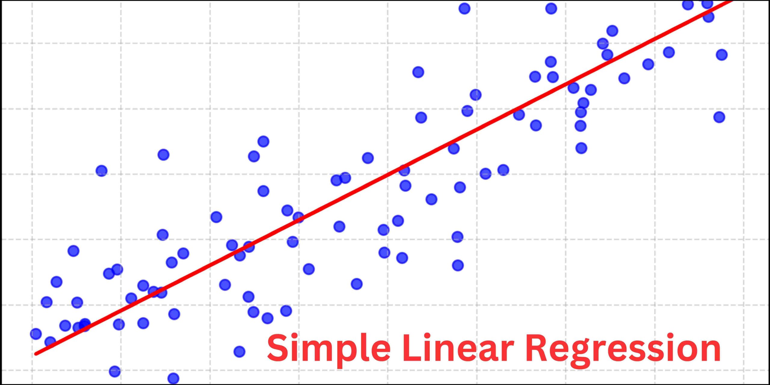
Simple linear regression is a statistical method for finding the relationship between an independent variable (predictor variable) and a dependent variable (response variable). Let’s try to comprehend simple linear regression with the help of an example.
Assume that you work as a data scientist for a real estate company and you want to find out how the selling price of a house depends on the area of the house. Here, the area of a house is the independent (predictor) variable, and the selling price is the dependent (response) variable. You can develop a simple linear regression model to find the relationship between the selling price of houses and the area of houses assuming a linear relationship exists between them.
We can implement simple linear regression in R or Python. We can use Scikit-learn or Statsmodels to implement simple linear regression in Python. If you want to implement simple linear regression in R, you can use the lm() function to fit a linear regression model.
I hope you have understood my explanation up to this point. Now, let us dig deep into the article to know how to implement simple linear regression in R. In the following sections, we will discuss various concepts of simple linear regression and how to implement simple linear regression in R.
Mathematical Foundation Of Simple Linear Regression
Let us assume a dataset consisting of one independent variable (x) and one dependent variable (y). We can express the relationship between x and y using simple linear regression as,
In the above equation, b0 is the intercept of the regression line, b1 is the slope of the regression line e is the error term which is the difference between the observed and predicted value of the dependent variable. The objective is to evaluate the values of b0 and b1 that will minimize the total error of the model.
Assumptions of Simple Linear Regression
The validity and reliability of simple linear regression depend on several assumptions.
Let us discuss them one by one briefly.
Linearity
The dependent variable (y) should be linearly related to the independent variable (x). One way to verify linear relationships is with the help of a scatter plot of the data points (x, y) and checking whether they fall along a straight line. If so then we have a linear relationship between x and y. On the other hand, if the scattered data points are forming a curve or a shape, then we don’t have linearity.
Independence
The assumption states that the residuals (difference between the observed value and predicted value of the dependent variable) should be independent of each other. Let us try to understand the independence assumptions with the help of a simple example.
Suppose we want to examine the relationship between the number of hours studied and exam scores of students. If the marks scored by students in a study group are interdependent then there is a violation of the independent assumption. This may happen if students in the same group share study materials or collaborate during exams which may lead to a correlation between their exam scores.
Therefore, before applying simple linear regression, we need to ensure that the observations in the dataset are independent of each other and are not affected by any external factors. In doing so, we will avoid violating the independence assumptions and obtain reliable and valid results from our analysis.
Normality
The normality assumption states that the residuals should follow a normal distribution (bell-shaped curve). Violation of normality assumption can lead to inaccurate results in simple linear regression. We can examine the normality condition with the help of a histogram or Q-Q plot of the residuals.
Statistical tests such as the Shapiro-Wilk test or the Kolmogorov-Smirnov test can also be used to check the null hypothesis that the residuals follow a normal distribution.
If the residual does not follow a normal distribution, we can normalize the data by transformation or use another non-parametric test.
Homoscedasticity
According to the homoscedasticity assumption, the variance of the residuals should not vary significantly as the value of the predictor variable changes. In other words, the variance of the error term should be approximately constant for simple linear regression.
We can check the homoscedasticity assumption, with the help of the scatterplot of the residuals against the dependent variable. For the Homoscedastic condition to be fulfilled, the residuals should show uniform dispersion along the horizontal axis.
The homoscedasticity assumption can also be checked with the help of various statistical tests such as the Breusch-Pagan test or White’s test.
Practical Implementation Of Simple Linear Regression In R
In this section, we will implement simple linear regression in R for predicting the salary based on years of experience. You can find the source code in the following link.
We have a dataset that has two columns: “YearsExperience” and “Salary”. Total number of rows in the dataset is 30. Here, “Salary” is the dependent variable, and “YearsExperience” is the independent variable.
Install Libraries
To implement simple linear regression in R, we need to install the “caTools”. This tool is popular for various data manipulation tasks such as sample splitting, data cleaning, and variable transformations.
install.packages('caTools')Import Dataset
Here, we will import the dataset from a CSV file. Below we show the dataset in the table for better understanding (Figure 1).
data = read.csv('Salary_DataSet.csv')
print(data)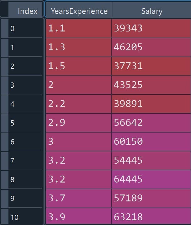
Figure 1: Salary dataset preview (YearsExperience vs Salary)
Split Dataset Into Training And Test Set
Here we will split the data into two parts: 75% of the data for training and 25% of the data for testing. To perform splitting, a variable named “SplitRatio” is defined that takes a value of 0.75. Note that sample.split is a function from the “caTools” package.
library(caTools)
set.seed(145)
split_data = sample.split(data$Salary, SplitRatio = 0.75)
train_data_set = subset(data, split_data == TRUE)
test_data_set = subset(data, split_data == FALSE)
Train A Simple Linear Regression Model
regressor = lm(formula = Salary ~ YearsExperience, data = train_data_set)Predicting Salaries Using Linear Regression Model
y_predict = predict(regressor, newdata = test_data_set)y_test=test_data_set$Salary
comparison <- cbind(y_predict, y_test)
print(comparison)The table below compares the predicted value (y_predict) of the dependent variable with its observed value (y_test).
The figure below (Figure 2) shows the predicted salary versus the observed salary in tabular form.
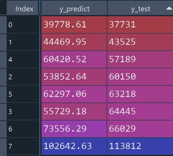
Figure 2: Predicted vs observed salary (tabular comparison)
Visualizing Model Performance on Training and Test Sets
#Create A Dataframe
plot_df=data.frame(YearsExperience = test_data_set$YearsExperience, ObservedSalary = test_data_set$Salary, PredictedSalary = y_predict)
print(plot_df)# Plot Regression Line With Respect To Observed Data points
library(ggplot2)
ggplot(plot_df, aes(x = YearsExperience, y = ObservedSalary)) +
geom_point(color = "darkcyan", size = 3) +
geom_line(aes(y = PredictedSalary), color = "red", size = 1.2) +
labs(title = "Simple Linear Regression",
x = "Years of Experience",
y = "Salary",
subtitle = "Observed Value vs. Predicted Value",
caption = "Source: Salary_DataSet.csv") +
theme_minimal() +
theme(plot.title = element_text(size = 18, face = "bold"),
axis.title = element_text(size = 14),
axis.text = element_text(size = 12),
plot.subtitle = element_text(size = 14),
plot.caption = element_text(size = 10),
panel.border = element_rect(color = "black", fill = NA, size = 1))The figure below (Figure 3) shows a graphical comparison of the observed salary and predicted salary values.
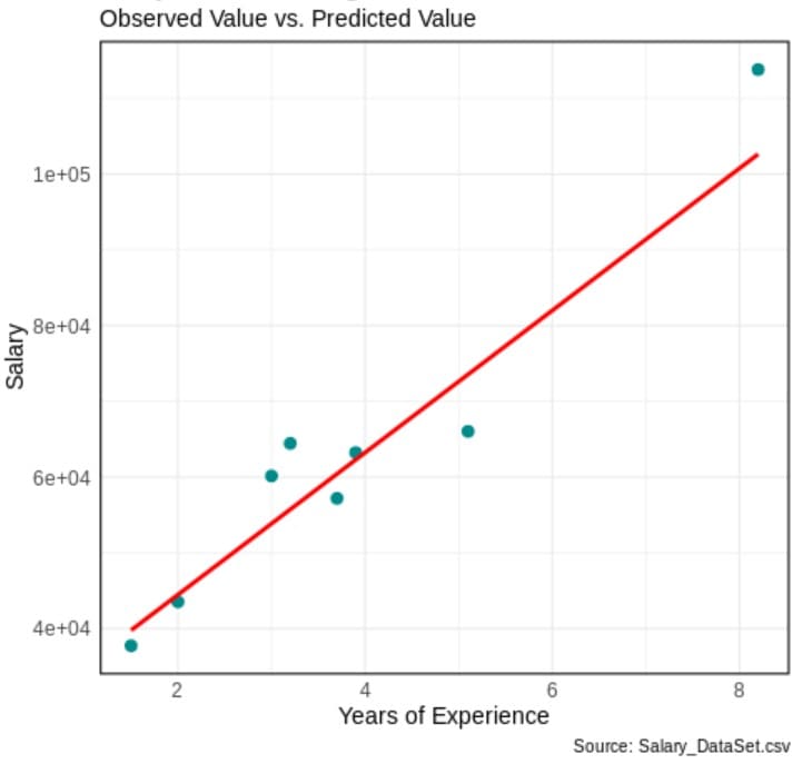
Figure 3: Observed salary vs predicted salary (regression line on test set)
Evaluate Performance Matrices
# Mean Squared Error (MSE)
mse <- mean((y_predict - y_test)^2)
cat("Mean Squared Error (MSE):", mse, "\n")# Root Mean Squared Error (RMSE)
rmse <- sqrt(mse)
cat("Root Mean Squared Error (RMSE):", rmse, "\n")# R Squared
r_squared <- 1 - mse / var(y_test)
cat("R-squared (R2):", r_squared, "\n")Conclusion
Simple linear regression is a popular statistical method for fitting the linear relationship between a dependent and an independent variable. In this article, we learned the mathematical foundation and various assumptions of simple linear regression.
We further applied simple linear regression in R to model the relationship between two variables: Year of experience and Salary. This involves, importing data from a CSV file, splitting the dataset to train and test sets, training a simple linear regression model, and evaluating model performances. We considered various performance metrics such as MSE, RMSE, and R-squared to evaluate the performance of the regression model.
Simple linear regression can be a valuable tool for statistical analysis in various fields, such as data science, artificial intelligence, statistical research, business, and predictive analysis. Implementing simple linear regression in R is quite straightforward, as R provides built-in functions such as lm() to perform the analysis quickly and efficiently. However, we should carefully consider various limitations and assumptions of simple linear regression while interpreting the results and model predictions.
Frequently Asked Questions
What is meant by simple linear regression?
Simple linear regression is a statistical method to find the relationship between two continuous variables by fitting a straight line to the data points. From the linear relationship, one can easily understand how the changes in one variable can affect the other. Simple linear regression is very popular for predicting outcomes and analyzing trends in various fields such as economics, social sciences, and healthcare.
What is the application of linear regression?
Linear regression is widely used across domains for predictive modeling and understanding relationships between variables. We can use linear regression to predict sales based on advertising expenditure, analyze trends in financial markets, optimize manufacturing processes by identifying factors affecting product quality, study economic relationships such as income and expenditure patterns, assess the impact of environmental factors on ecological variables, etc.
References
Simple Linear Regression Model
[Correlation And Simple Linear Regression](http://Correlation and Simple Linear Regression)