Overview
Have you ever wondered how to use a pre-trained model such as ResNet50 to enhance the performance of your machine learning projects? If that’s the case, this article is meant for you.
In this article, you will learn how to perform transfer learning using Keras and ResNet50, which is a popular pre-trained convolutional neural network (CNN) architecture.
This article starts with the basic introduction of ResNet and transfer learning. After that, you will learn how to apply the transfer learning model using resnet50 and Keras to classify the CIFAR-10 dataset. You will learn various essential steps of transfer learning such as how to freeze layers of a ResNet50 model, how to add new trainable layers, and how to fine-tune the model.
It does not matter whether you are a beginner or advanced user of AI &ML; this article will help you immensely to accelerate your machine learning projects.
What Is ResNet?
ResNet is an innovative CNN architecture proposed by Microsoft researchers in 2015. It won the ImageNet competition in 2015 by a significant margin while achieving the top-5 error rate of just 3.57%.
With the use of ResNet, one can easily develop deep neural networks with many layers ranging from 18 to 152 layers without sacrificing performance. The secret is the skip connections in ResNet, which allow a seamless flow of information across various layers.
Prior to ResNet, deep learning models often suffered from vanishing and exploding gradient problems. ResNet mitigated these issues by using residual connections (skip connections).
We can use ResNet for various tasks, such as image classification, object detection, segmentation, facial recognition, transfer learning, and medical imaging. Some of the popular ResNet architectures are: ResNet-18, ResNet-34, ResNet-50, ResNet-101, and ResNet-152. In this article, we will use ResNet-50 as a base model for transfer learning on the CIFAR-10 dataset.
The figure below (Figure 1) shows a pictorial representation of ResNet architecture. Here, we won’t be explaining the network. Interested readers can learn more about the ResNet architecture from my previous blog post.
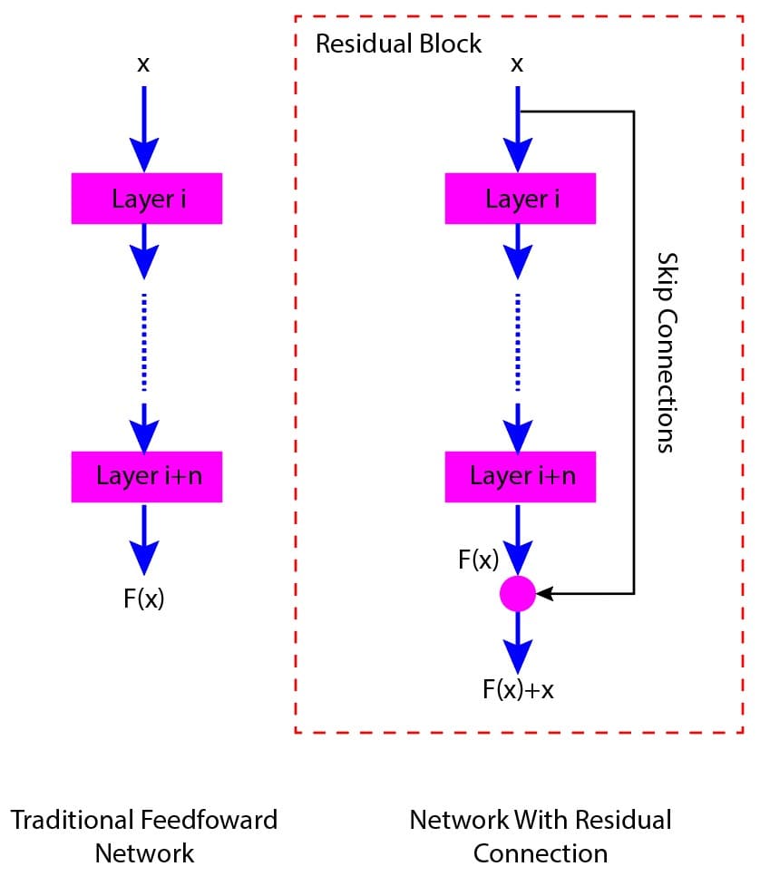
Figure 1: Pictorial representation of ResNet with skip (residual) connections
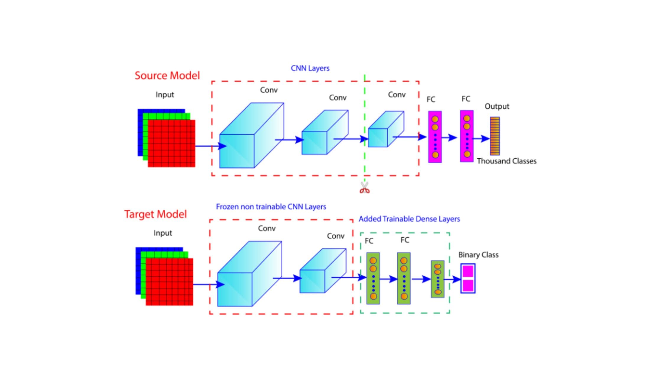
What Is Transfer Learning
Transfer learning is a popular method in deep learning that allows the use of features learned from one task and apply them to a related task. In transfer learning, a pre-trained model designed for a specific task is adapted to a new but similar task.
Let us illustrate transfer learning with the help of an analogy. Assume that you are a skillful tennis player. You have developed various skills, such as honing excellent hand-eye coordination, agility, and strategic thinking by playing tennis.
Now, if you want to play badminton, you do not need to start from scratch. Many of the fundamental skills that you learned while playing tennis can help you immensely to quickly learn badminton without any racquet sports experience.
A similar concept applies in transfer learning, where a model trained on one task, such as recognizing objects in photos, can be adapted to perform a related but different task, such as identifying specific types of objects.
Practical Implementation
Here, we will develop a transfer learning model using resnet50 and Keras to classify the CIFAR-10 dataset.
Import Necessary Libraries
from keras.datasets import cifar10
from sklearn.model_selection import train_test_split
from keras.utils import to_categorical
from keras.applications.resnet50 import ResNet50, preprocess_input
from keras import models
from keras import layers
from keras import optimizers
import tensorflow as tf
import matplotlib.pyplot as plt
Data Processing
Load Data
Here, the CIFAR-10 dataset is loaded and split into training and test sets.
(x_train, y_train), (x_test, y_test) = cifar10.load_data()Here, we printed the shape of the data arrays to understand their dimension. The training set contains 50000 images and the test set contains 10000 images.
print(x_train.shape)
print(x_test.shape)Output:
(50000, 32, 32, 3)
(10000, 32, 32, 3)print(y_train.shape)
print(y_test.shape)Output:
(50000, 1)
(10000, 1)Normalize The Data
Each pixel in the image has a value between 0 and 255, representing the intensity of that color channel. Here, we divide the pixel values by 255. This normalizes the data from the original range of [0, 255] to a new range of [0, 1].
x_train = x_train / 255.0
x_test = x_test / 255.0
Convert The Categorical Labels To One-hot Encoded Vectors
The CIFAR-10 dataset contains ten different classes of images: Airplane, Automobile (Car), Bird, Cat, Deer, Dog, Frog, Horse, Ship, and Truck. The labels for these classes are originally represented as integers from 0 to 9. For example, if an image is of a car, its label might be 3.
Here, we perform One-hot encoding that converts class labels into one-hot encoded vectors.
y_train = to_categorical(y_train, 10)
y_test = to_categorical(y_test, 10)print(y_train.shape)
print(y_test.shape)Output:
(50000, 10)
(10000, 10)Split Training Data Into Train And Validation sets
Here, we split the training data into training and validation sets using the “train_test_split” function.
x_train, x_val, y_train, y_val = train_test_split(x_train, y_train, test_size=0.1, random_state=42)Loading The Pre-trained ResNet50 Model
Let us initialize the pre-trained ResNet50 model with specific configurations. Here, weights=’imagenet’ specifies that the model should be initialized with weights pre-trained on the ImageNet dataset.
Moreover, “include_top=False”, indicates that the fully connected (dense) layers at the top of the network should not be included.
base_model=ResNet50(weights='imagenet', include_top=False, input_shape=(224, 224, 3))We can check all the layers of the base_model using the following command.
base_model.summary()Build Model
Here we construct a neural network model using the Keras Sequential API.
#Create A Sequential Model
model = models.Sequential()
The CIFAR-10 images are 32×32 however, the ResNet50 expects 224×224. Hence, we here performed upsampling that scales up the 32×32 images to 224×224, matching the input shape expected by ResNet50.
# Add A UpSampling2D Layer
model.add(layers.UpSampling2D((7, 7)))
The code below adds the pre-trained ResNet50 model initialized earlier with include_top=False.
#Add ResNet50 As Base Model
model.add(base_model)
Now, we can add custom layers on the top.
# Add GlobalAveragePooling2D Layer
model.add(layers.GlobalAveragePooling2D())# Add A Output Layer
model.add(layers.Dense(10, activation='softmax'))Compile The Model
Compile the model with a learning rate of 1e-4. Here, we used the categorical cross-entropy as a loss function. This type of loss function is suitable for multi-class classification problems where the labels are one-hot encoded.
model.compile(optimizer=optimizers.RMSprop(learning_rate=1e-4), loss='categorical_crossentropy', metrics=['acc'])Train The Model
Now let us train the model for 5 epochs.
with tf.device('/device:GPU:0'):
      history = model.fit(x_train, y_train, epochs=5, batch_size=20, validation_data=(x_val, y_val))
Evaluate The Model Performance
model.evaluate(x_test, y_test)Visualize The Model Performance
# Plot training & validation accuracy values
plt.figure(figsize=(12, 4))

plt.plot(history.history['acc'])
plt.plot(history.history['val_acc'])
plt.title('Model accuracy')
plt.ylabel('Accuracy')
plt.xlabel('Epoch')
plt.legend(['Train', 'Validation'], loc='upper left')
The figure below (Figure 2) illustrates model accuracy with respect to the number of epochs.
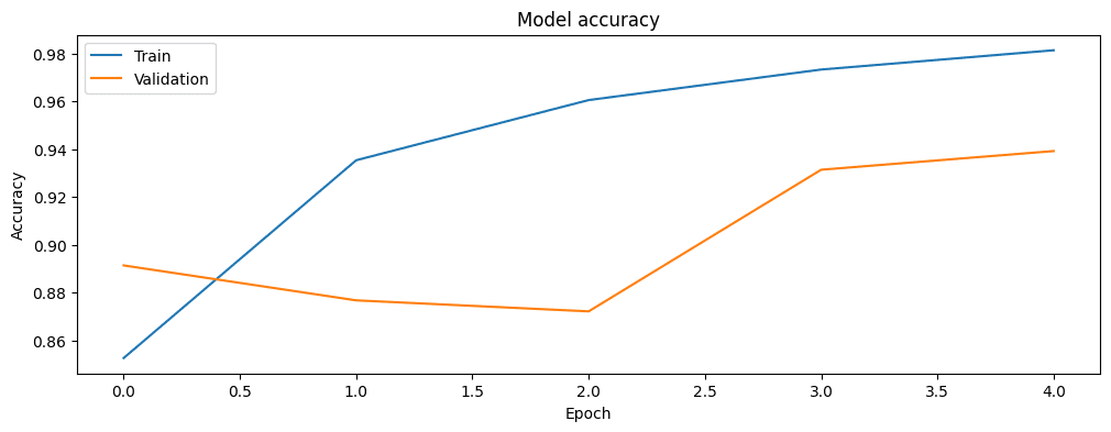
Figure 2: Model accuracy with respect to the number of epochs
# Plot training & validation loss values
plt.plot(history.history['loss'])
plt.plot(history.history['val_loss'])
plt.title('Model loss')
plt.ylabel('Loss')
plt.xlabel('Epoch')
plt.legend(['Train', 'Validation'], loc='upper left')

plt.show()
The figure below (Figure 3) illustrates model losses with respect to the number of epochs.
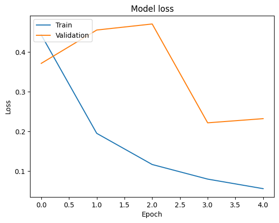
Figure 3: Model losses with respect to the number of epochs
Fine Tuning
Let us unfreeze some of the layers for fine-tuning. Here, fine_tune_at = 100 means that layers before the 100th layer of the model will be frozen (i.e., their weights will not be updated during training), while layers from the 100th layer onward will be unfrozen and trained.
# Unfreeze Some Layers In The Convolutional Base For Fine-tuning
base_model.trainable = True
fine_tune_at = 100 # Unfreeze from this layer onwards# Compile The Model
model.compile(optimizer=optimizers.RMSprop(learning_rate=1e-4), loss='categorical_crossentropy', metrics=['acc'])# Train The Model
history_fine = model.fit(x_train, y_train, epochs=5, batch_size=20, validation_data=(x_val, y_val))Output:
Epoch 1/5
2250/2250 [==============================] - 512s 219ms/step - loss: 0.0457 - acc: 0.9843 - val_loss: 0.2353 - val_acc: 0.9360
Epoch 2/5
2250/2250 [==============================] - 492s 219ms/step - loss: 0.0364 - acc: 0.9879 - val_loss: 0.3803 - val_acc: 0.9180
Epoch 3/5
2250/2250 [==============================] - 488s 217ms/step - loss: 0.0342 - acc: 0.9888 - val_loss: 0.2350 - val_acc: 0.9424
Epoch 4/5
2250/2250 [==============================] - 493s 219ms/step - loss: 0.0264 - acc: 0.9913 - val_loss: 0.2417 - val_acc: 0.9402
Epoch 5/5
1694/2250 [=====================>........] - ETA: 1:56 - loss: 0.0235 - acc: 0.9919# Evaluate The Model
model.evaluate(x_test, y_test)Conclusions
In this article, we learned how to apply transfer learning with the ResNet50 model on the CIFAR-10 dataset. The findings suggest the very good performance of our model in classifying the CIFAR-10 dataset.
We further fine-tuned the model and achieved even better performance, highlighting the effectiveness of this approach.
The use of ResNet50 with transfer learning has its practical benefits, especially with smaller datasets. The combination of a strong pre-trained model and fine-tuning can be a valuable strategy for machine learning projects. Embracing these techniques can help you achieve superior outcomes and streamline the development process in the dynamic field of AI.
Frequently Asked Questions
What is the image size for ResNet50?
The image size of Resnet50 is 224 x 224 pixels.
How many layers are there in ResNet50?
Resnet50 consists of 50 layers.
What is the difference between CNN and ResNet?
Convolution neural networks (CNNs) are deep learning models that are designed to process structured grid data such as images. They use convolutional layers to detect patterns. On the other hand, the ResNet is a specific type of CNN with skip connections or residual connections. This helps to mitigate the vanishing gradient problem and allows the training of much deeper networks.
References And Related Article
Unleashing ResNet: A Game-Changer In Deep Learning