Overview
In this article, we will learn polynomial regression and its practical implementation in Python. It is a supervised approach where non-linear relationships between dependent and independent variables are modeled with the help of a polynomial function. We can use polynomial regression to analyze non-linear data, such as curves, growth rates, disease outbreaks, etc.
For example, the spread rate of infectious diseases (such as COVID-19), which is highly non-linear with time, can be fitted with the help of polynomial regression. In this article, we will learn various concepts of polynomial regression and its practical implementation in Python.
If you want to start with the fundamentals, you can also check out our Simple Linear Regression article.
Why Use Polynomial Regression?
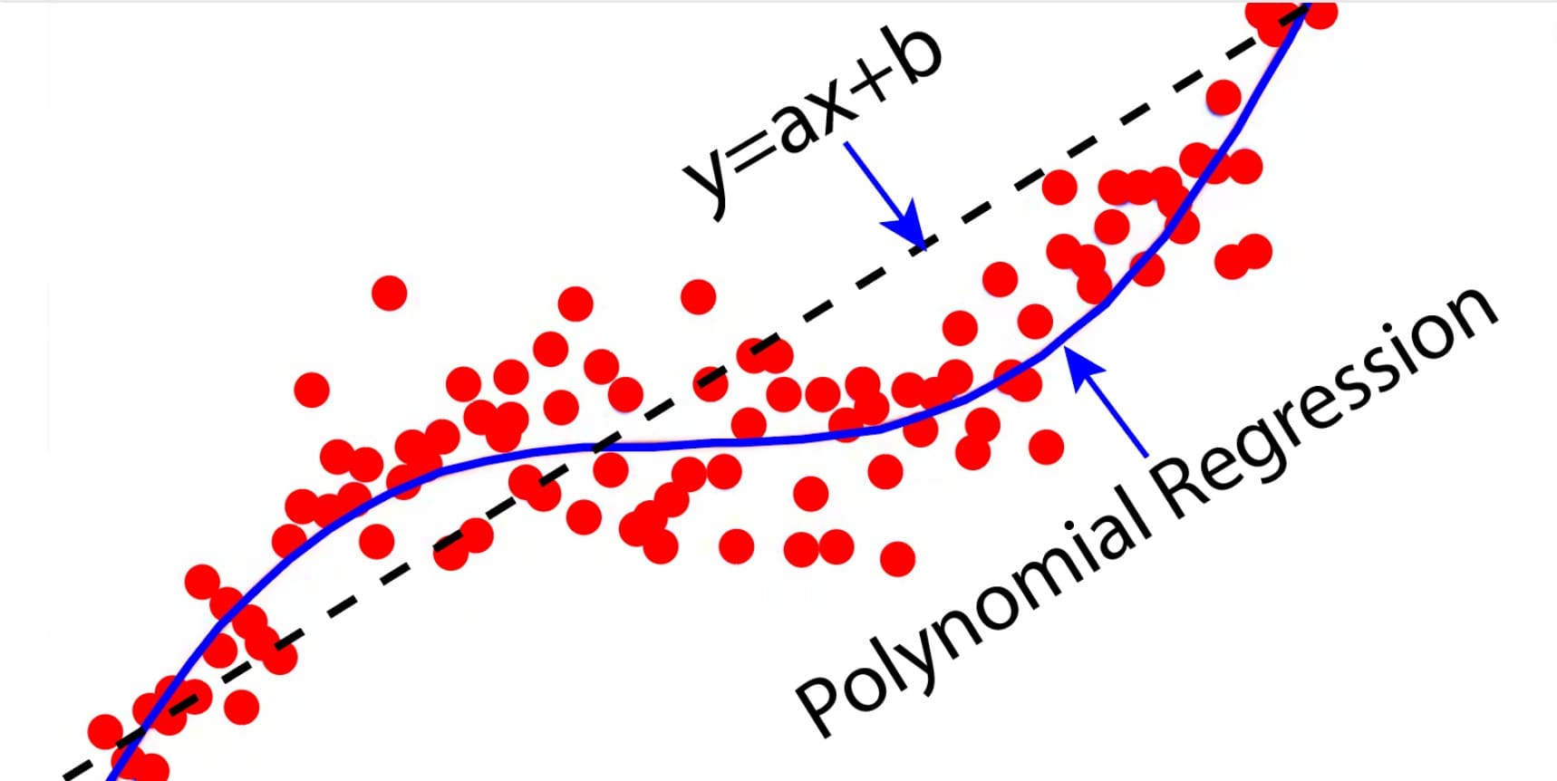
Linear regression generally fails to model non-linear data. Instead, we can use polynomial regression to fit non-linear variables with the help of polynomial functions. Let us try to understand the difference between polynomial and linear regression with the help of Figure 1.
The figure illustrates the relationship between two variables, X and Y. It shows that the linear regression plot (a straight line) seems to be a very poor fit for the nonlinear scattered data. However, the polynomial regression plot (curvilinear plot) approximates the scattered data better. Hence, we need to use Polynomial regression to fit non-linear data.
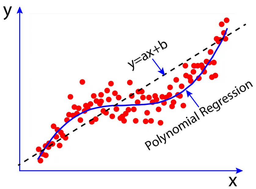
Figure 1: Polynomial regression fits non-linear data better than simple linear regression
What Is Polynomial Regression?
In the case of linear regression, the relationship between dependent and independent variables can be expressed using a linear equation:
Here, y is the dependent variable, x is the independent variable, and b is the coefficient.
For non-linear data, we need to modify the linear equation by including higher-order terms of x. As an illustration, we can introduce a quadratic term into the linear equation to account for a non-linear relationship.
We can further modify the equation by including cubic, quartic, or other higher-order terms depending on the complexity of dependent and independent variables. This will lead us to the general form of the polynomial regression equation.
Feature Transformation
Polynomial regression uses polynomial features, which are a type of feature engineering in machine learning models, to capture nonlinear relationships between the dependent and independent variables. With the help of feature transformation, the original features of datasets are transformed into polynomial features of the required degree, allowing the capture of non-linear relationships between variables.
Suppose we have a dataset with a non-linear relationship between input feature x and output feature y. We want to find the relationship between x and y with the help of polynomial regression of degree 3. To do this, we have to create new features such as x2 and x3 from existing feature x. We then add the new features to the original dataset to create a transformed version of x. The transformed version allows us to consider the original features, their interactions, and higher-order terms. By doing so, it becomes capable of fitting nonlinear relationships in the data.
Practical Implementation
Here, we provided two examples of polynomial curve fitting (regression) in Python using the scikit-learn library. The codes and dataset are found in the following links: Ex1, Ex2, dataEx1, and dataEx2.
To make the ideas more concrete, let us implement polynomial regression step by step.
Example 1
In the first example, we want to predict the salaries of employees based on their level in the company.
The table shows the different job positions, their levels, and corresponding salaries. The table has four columns: Index, Position, Level, and Salary. We will use the ‘Level’ column as the independent variable and the ‘Salary’ column as the dependent variable.
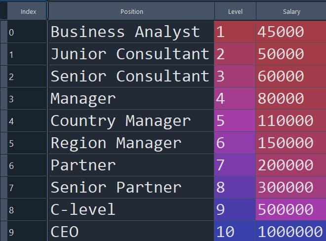
Figure 2: Visual depiction of the dataset for Example 1
Import Necessary Libraries
import numpy as np
import pandas as pd
import matplotlib.pyplot as plt
Read Dataset From CSV File Using Pandas
df=pd.read_csv("Position_Salaries.csv")
X = df.iloc[:, 1:-1].values
y = df.iloc[:, -1].values
Fit Linear Regression Model
We here develop a linear regression using the scikit-learn library.
from sklearn.linear_model import LinearRegression
Linear_Regressor=LinearRegression()
Linear_Regressor.fit(X,y)
Visualize Linear Regression Results
plt.scatter(X,y, color='Red')
plt.plot(X, Linear_Regressor.predict(X), color='blue')
plt.title("Plot Of Linear Regression")
plt.xlabel("Position Level")
plt.ylabel("Salaries")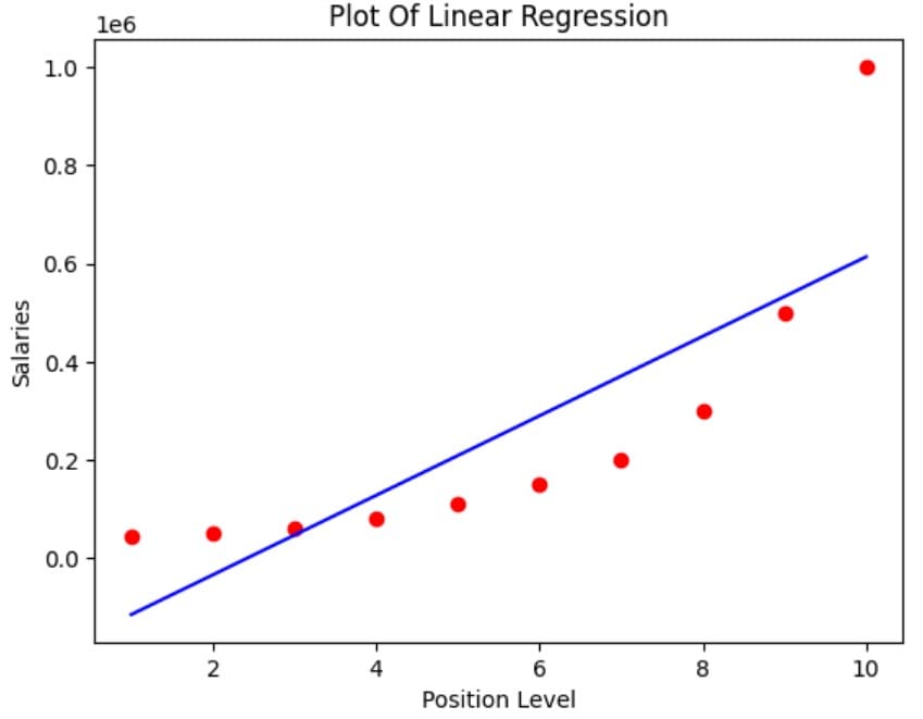
Figure 3: Simple linear regression plot for Example 1
Fit Polynomial Regression Model
# Perform Polynomial Transformation
from sklearn.preprocessing import PolynomialFeatures
Poly_Transformer=PolynomialFeatures(degree=6)
X_Transform=Poly_Transformer.fit_transform(X)# Fit Model
Lin_regressor2=LinearRegression()
Lin_regressor2.fit(X_Transform,y)Visualize Regression Results
plt.scatter(X, y, color='red')
plt.plot(X, Lin_regressor2.predict(Poly_Transformer.fit_transform(X)), color='black' )
plt.title("Results Of Polynomial Regression")
plt.xlabel('Position Level')
plt.ylabel('Salaries')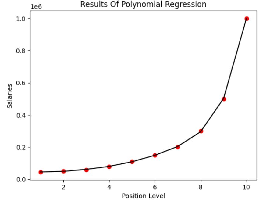
Figure 4: Polynomial regression plot for Example 1
Prediction For Sample Data
# Prediction Of New Results With Linear Regressors
print(Linear_Regressor.predict([[6.5]]))330378.78787879# Prediction Of New Results With Polynomial Regressor
print(Lin_regressor2.predict(Poly_Transformer.fit_transform([[6.5]])))174192.81930595Example 2:
Here, we will develop another regression model with multiple independent variables. This problem has three independent variables (TV, radio, newspaper) and one dependent variable (sales). Our aim is to find the relationship between the independent and dependent variables. The dataset consists of 200 rows and 4 columns. In the table below, we have shown the partial datasets for visualization of the data.
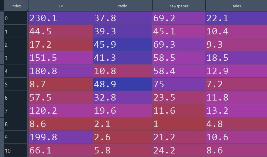
Figure 5: Visual depiction of the dataset for Example 2
Read Data From CSV File Using Pandas
df = pd.read_csv("Advertising.csv")X = df.iloc[:, :-1].values
y = df.iloc[:, -1].valuesPerform Polynomial Transformation
from sklearn.preprocessing import PolynomialFeatures
polynomial_transformer = PolynomialFeatures(degree=2,include_bias=False)
X_transform = polynomial_transformer.fit_transform(X)
If you want to learn regression with multiple independent variables in detail, you can also check our Multiple Linear Regression article.
Perform Regression
# Train Test Split
from sklearn.model_selection import train_test_split
X_train, X_test, y_train, y_test = train_test_split(X_transform, y, test_size=0.3, random_state=101)
from sklearn.linear_model import LinearRegression
model = LinearRegression(fit_intercept=True)# Fit model
model.fit(X_train,y_train)# Model Prediction
model_predictions = model.predict(X_test)
print(model_predictions)[13.94856153 19.33480262 12.31928162 16.76286337 7.90210901 6.94143792
20.13372693 17.50092709 10.56889 20.12551788 9.44614537 14.09935417
12.05513493 23.39254049 19.67508393 9.15626258 12.1163732 9.28149557
8.44604007 21.65588129 7.05070331 19.35854208 27.26716369 24.58689346
9.03179421 11.81070232 20.42630125 9.19390639 12.74795186 8.64340674
8.66294151 20.20047377 10.93673817 6.84639129 18.27939359 9.47659449
10.34242145 9.6657038 7.43347915 11.03561332 12.65731013 10.65459946
11.20971496 7.46199023 11.38224982 10.27331262 6.15573251 15.50893362
13.36092889 22.71839277 10.40389682 13.21622701 14.23622207 11.8723677
11.68463616 5.62217738 25.03778913 9.53507734 17.37926571 15.7534364 ]# Compute MAE, MSE and RMSE
from sklearn.metrics import mean_absolute_error,mean_squared_error
MAE = mean_absolute_error(y_test,model_predictions)
MSE = mean_squared_error(y_test,model_predictions)
RMSE = np.sqrt(MSE)
print("MAE:",MAE )
print("MSE:",MSE )
print("RMSE:",RMSE )MAE: 0.4896798044803838
MSE: 0.4417505510403753
RMSE: 0.6646431757269274Limitations
The following are the limitations of the polynomial regression:
-
Overfitting: Overfitting happens when the model fits training data well but makes poor predictions on new data. We may often encounter overfitting issues when dealing with higher-order polynomials.
-
Poor Extrapolation: The model may perform poorly in predicting values outside the range of training data. Hence, exploration outside the range should be avoided.
-
Presumption Of Polynomial Relationship: In polynomial regression, we assume a polynomial relationship between dependent and independent variables. However, the model may perform poorly if the relationship between dependent and independent variables is not polynomial.
-
Computational Complexity: Polynomial regression with a high degree of polynomial on large datasets can be computationally expensive.
-
Decreased Interpretability: This type of model may become highly complex and difficult to interpret as the degree of polynomial increases.
Conclusions
-
With the help of polynomial regression, we can analyze non-linear data such as curves, growth rates, and disease outbreaks. It is a powerful supervised learning method for predictive analytics and understanding complex patterns in non-linear data.
-
Polynomial regression in machine learning can accurately model non-linear data using higher-order terms of independent variables.
-
In this article, we learned how to use scikit-learn to implement polynomial regression in Python.
Frequently Asked Questions
When should I use polynomial regression?
Polynomial regression is ideal when the relationship between the independent and dependent variables is non-linear in nature. For example, we can use polynomial regression to analyze the spread of infectious diseases in populations, model sediment isotope studies, and understand complex trends of data in various organization sectors that linear models fail to capture accurately.
What is the difference between linear and polynomial regression?
The differences between polynomial and linear regression are in how they model the relationship between variables. Linear regression is used to fit a linear relationship between the dependent and independent variables using a straight-line equation. On the other hand, polynomial regression can fit complex data patterns using a polynomial equation, allowing curves and bends in the relationship.
What is a polynomial regression?
Polynomial regression is a statistical method used to model nonlinear relationships between dependent and independent variables. Unlike linear regression, which fits data to a straight line, polynomial regression employs polynomial equations to fit data. This allows polynomial regression to capture complex data patterns involving curves and bends in the relationship.
References
Regression in machine learning
