Overview
Multiple linear regression is a popular statistical method for finding the relationship between multiple independent variables (also known as predictor variables) and one dependent variable (response variable). For example, we can apply multiple linear regression to find the relationship between multiple independent variables such as the age of persons, gender, educational qualifications, and income with the yearly expenditure of the person.
Multiple linear regression can handle multiple independent variables, unlike simple linear regression which can handle only one independent variable. In a real-world scenario, multiple factors generally influence a single outcome, making multiple linear regression a more appropriate approach.
In this article, we will learn the theories of multiple linear regression and its practical implementation in Python. We will use the scikit-learn library to train a multiple linear regression model on sample datasets and evaluate its performance to make predictions on unseen new data.
The Equation of Multiple Linear Regression
Let us consider a simple example to understand the equation of multiple linear regression. In the example, there are 100 observations (rows) with three independent variables: area (floor area), bedrooms (number of bedrooms), and age (age of house).
We can write the following equation to predict the price of the house based on area, bedrooms, and age.
We can write the above equation in a more general form as,
In the above equation, y is the dependent (response) variable, x1, x2,…..xn are the independent variable (predictor variable), b0 is the intercept, e is the error term (difference between observed value and predicted value of the dependent variable)
Assumptions Of Multiple Linear Regression
There are several assumptions of multiple linear regression that need to be met to ensure the validity of the model and the accuracy of the results. Let us discuss those one by one:
Linear Relationship
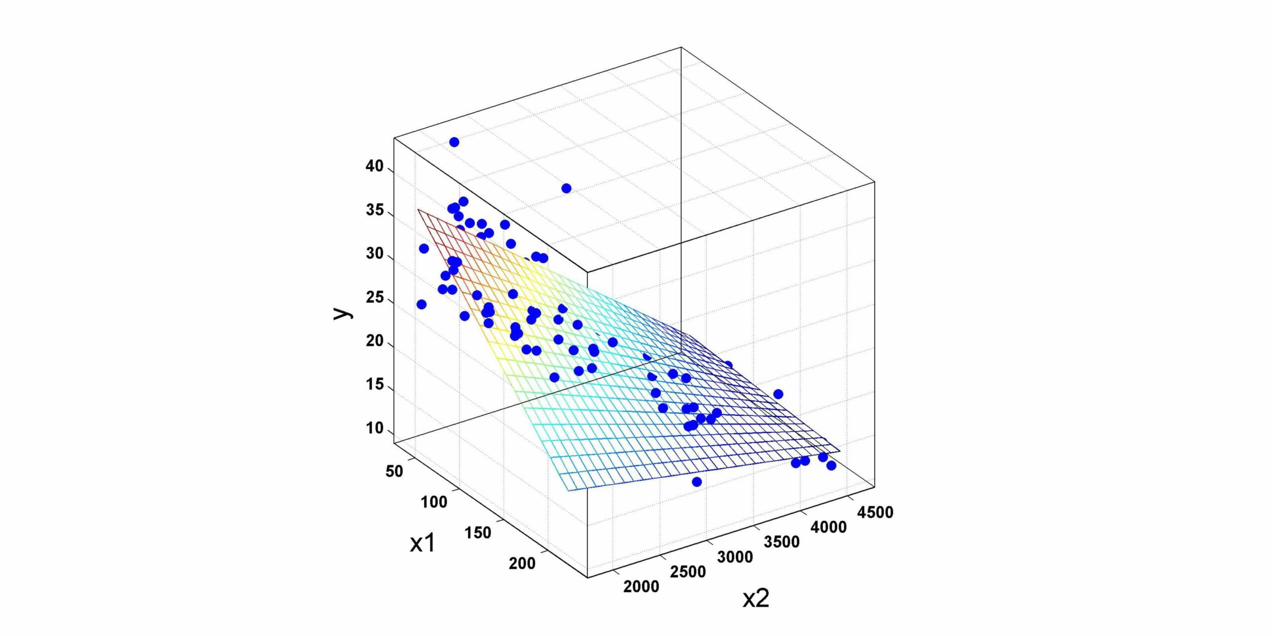
Multiple linear regression assumes a linear relationship between the independent (predictor) and dependent (response) variables. We can visually inspect the linear relationship with the help of a scatter plot of independent and dependent variables. As a general rule, the scattered data points should fall along a straight line, if there is any linear relationship among the variables.
No Multicollinearity
The independent (predictor) variables should not be highly correlated with each other in multiple linear regression. We can detect multicollinearity with the help of variance inflation factor (VIF) or correlation matrix. In general, the VIF value of 1 indicates no multicollinearity in the dataset.
However, the VIF value greater than 5 or 10 indicates a major multicollinearity issue. The value of VIF less than 1 indicates a negative correlation between independent variables. Nevertheless, it is very rare in practice since the independent variables tend to have some degree of positive correlation with each other.
Multivariate Normality
In multiple linear regression, the distribution of the residuals should be symmetric and bell-shaped like the normal distribution. There are several ways to check the normality of the residuals such as the Shapiro-Wilk test, histogram, or Q-Q plot.
If the residuals are not normal then we can apply several measures such as removing outliers, transforming the dependent variable, or using a different model instead of multiple linear regression.
Homoscedasticity
Homoscedasticity is an important assumption in multiple linear regression that states how residuals (the difference between the observed and predicted values) of the dependent variable are distributed in the regression model.
The homoscedasticity condition ensures that the variance of the residuals of the dependent variable should be constant across all levels of independent (predictor) variables. There are several ways to check homoscedasticity such as residual plots or statistical tests such as the Breusch-Pagan test and the White test.
Independence
In multiple linear regression, the observations in the datasets should be independent of each other. In other words, the residuals of the model should not be correlated with each other. We may encounter, biased and inaccurate estimates of the regression coefficient in multiple linear regression if the datasets do not satisfy the independence assumption.
We may encounter a violation of the independence assumptions while fitting multiple linear regression models on time series data or clustered data. The time series data are collected over time and may exhibit autocorrelation. For clustered data, observations within the same clusters can be quite similar to each other than the observations from different clusters.
We can identify the validity of the independent assumptions in multiple linear regression with the help of several diagnostic tools and tests such as residual plots, autocorrelation plots Durbin-Watson Test, Time Series Analysis, and Ljung-Box Test.
Outlier Check
Outliers are the data points that are significantly different from the rest of the data in the dataset. The presence of outliers can significantly degrade the performance of the regression model. Outliers in the dataset can lead to increased model complexity, inaccurate estimation of performance metrics, and inaccurate model interpretation
We can check the presence of outliers in the dataset using various methods such as detecting outliers such as visual inspection of scatter plots, box plots, and residual plots. Once detected, the outliers can either be removed from the dataset or transformed to reduce their impact on the model.
We can also summarize various assumptions of multiple linear regression discussed above with the help of the following diagram below. The diagram below shows six concepts that should be met for multiple linear regression: linearity, homoscedasticity multivariate normality, independence, lack of multicollinearity, and the outlier check. In the figure, each concept is illustrated with the help of two examples: one that satisfies the assumption and one that violates the assumptions.
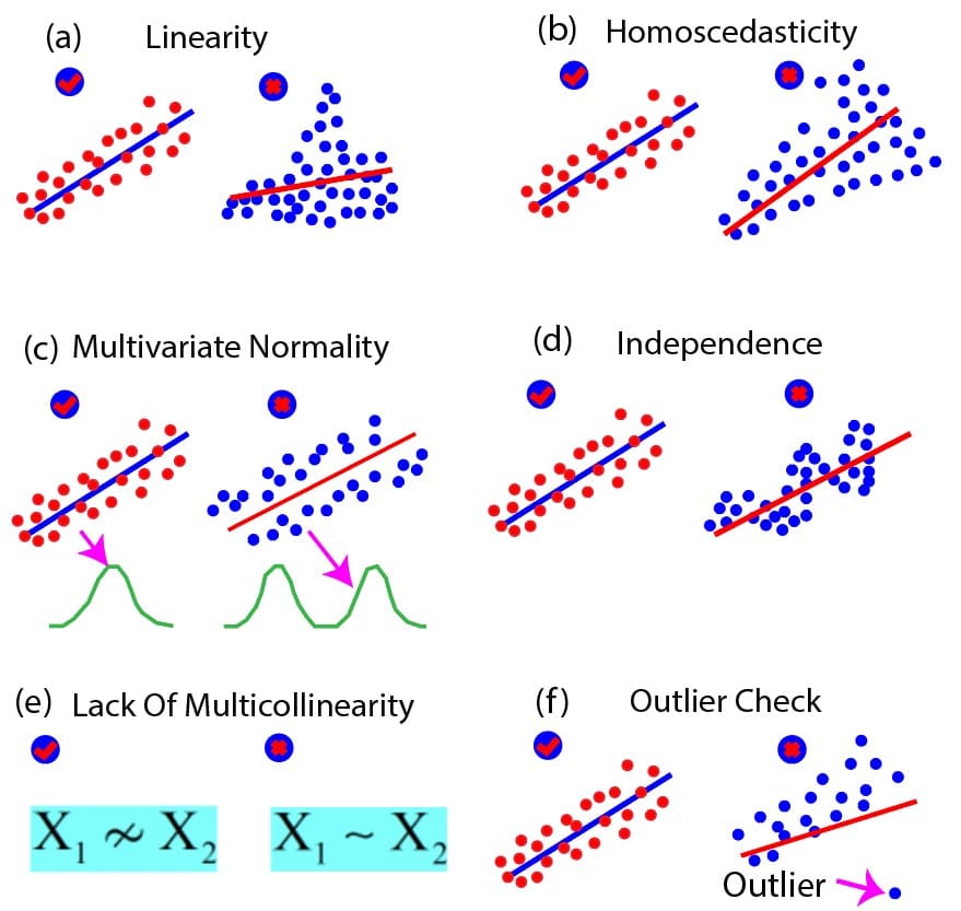
Figure 1: Summary of key assumptions of multiple linear regression (examples of satisfied vs violated assumptions)
Implementing Multiple Linear Regression in Python
In this section, we will implement Multiple Linear Regression in Python using the Scikit-learn library. You can find the code and dataset in the following link: Code and Dataset.
Import Necessary Libraries
import numpy as np
import pandas as pd
import matplotlib.pyplot as plt
from sklearn.preprocessing import OneHotEncoder
from sklearn.compose import ColumnTransformer
Import Datasets From A CSV File
We have a startup dataset in a CSV file that contains the following columns: R&D Spend, Administration, Marketing Spend, State, and Profit. Among them, Profit is the dependent variable and the rest of them are independent variables. Here we will load the data in the pandas data-frame from the CSV file.
df = pd.read_csv('StartupData.csv')
X = df.iloc[:, :-1].values
y = df.iloc[:, -1].values
We can visualize the data in the table below. There are 50 rows in the dataset.
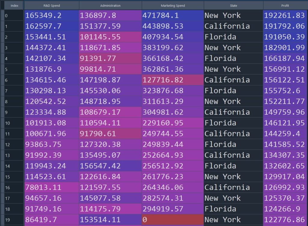
Figure 2: Startup dataset (sample rows) used for multiple linear regression
Categorical Data Encoding
As we can see, the fourth column {“State”} is categorical data. We need to transform the categorical data into a numerical format for using it as an independent (predictor) variable in the regression model. Here will will use one-hot encoding for categorical data encoding.
CT = ColumnTransformer(transformers=[('encoder', OneHotEncoder(), [3])], remainder='passthrough')
X = np.array(CT.fit_transform(X))
Split The Data Into Train and Test sets
Here we used the train_test_split function, to split the dataset into training and testing sets. We considered 75% of the data for training and 25% of the data for testing.
from sklearn.model_selection import train_test_split
X_train, X_test, y_train, y_test = train_test_split(X, y, test_size = 0.25, random_state = 0)
Train A Multiple Linear Regression Model
from sklearn.linear_model import LinearRegression
model = LinearRegression()
model.fit(X_train, y_train)
Model Prediction For Test Set
y_pred = model.predict(X_test)df = pd.DataFrame({'y_test': y_test, 'y_pred': y_pred})
print(df)The table below compares the value of the observed value of the dependent variable (y_test) with the predicted value of the dependent variable (y_pred). As we can see, the regression model seems to be performed very well in predicting the dependent variable.
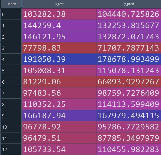
Figure 3: Observed (y_test) vs predicted (y_pred) values for the test set
Evaluate Performance Metrics
Here, we will use several metrics to evaluate the performance of the multiple linear regression model. These metrics help us to understand performance and accuracy of the regression model.
from sklearn import metrics# Compute Mean Absolute Error (MAE)
mae = metrics.mean_absolute_error(y_test, y_pred)
print('Mean Absolute Error::', mae)Mean Absolute Error:: 7024.5399# Compute Mean Squared Error (MSE)
mse = metrics.mean_squared_error(y_test, y_pred)
print('Mean Squared Error::', mse)Mean Squared Error:: 73809312.8822# Compute Root Mean Squared Error (RMSE)
rmse = np.sqrt(mse)
print('Root Mean Squared Error::', rmse)Root Mean Squared Error:: 8591.2346# Compute R-squared Score
r2 = metrics.r2_score(y_test, y_pred)
print('R-squared score::', r2)R-squared score:: 0.9315Conclusion
In this article, we provide a comprehensive explanation of the various assumptions of multiple linear regression along with mathematical details. Additionally, we developed a multiple linear regression model using Python to fit the relationship between the profit of a startup with R&D spending, administration, marketing spending, and state.
We further evaluated the performance of the model using various matrices such as mean squared error (MSE), root mean squared error (RMSE), and r-squared. These metrics can give a fair idea of the accuracy, effectiveness, and predictive capabilities of the multiple linear regression model
Multiple linear regression can be applied to fit the relationship between a dependent variable and multiple independent variables across different sectors such as finance, marketing, economics, healthcare, environmental science, and social science. The knowledge gained from this article can serve as a foundation for professionals seeking to harness the power of multiple linear regression in their respective domains.
Frequently Asked Questions
What is a multiple linear regression?
Multiple linear regression is a statistical method that finds the relationship between a single dependent variable and two or more independent variables. This method involves multiple independent variables, unlike simple linear regression, which has only one independent variable.
What is the difference between simple and multiple linear regression?
Simple linear regression is used to find the relationship between one dependent variable and one independent variable. On the other hand, multiple linear regression is used to find the relationship between one dependent variable and two or more independent variables. With the help of multiple linear regression, we can analyze the combined effect of several predictors on the outcome.
Why use multiple regression analysis?
Multiple regression analysis is used to find the relationship between one dependent variable and multiple independent variables. This helps to determine how much each predictor affects the outcome, how to improve the accuracy of predictions by taking multiple factors into account, and how to control for other influencing variables, giving a clearer understanding of the underlying relationships.
References
Multiple Linear Regression Quick Guide
Multiple Linear Regression: Basics
If you want to know simple linear regression then please check this article : Simple Linear Regression