Overview
Are you interested in developing a deep learning model to classify handwritten digits? If so, then this blog post is for you. Here, we will show you how to develop a deep learning model based on LeNet5 (LeNet) architecture to classify the MNIST dataset. We will use Keras, which is a high-level API for deep learning for developing a convolutional neural network model based on the LeNet5 architecture. We will use the MNIST dataset that contains 70000 images of handwritten digits within the range [0-9].
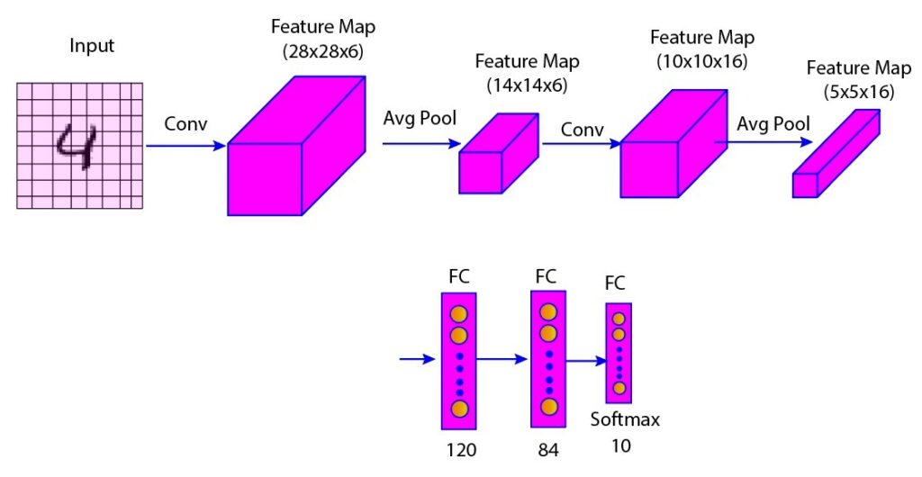
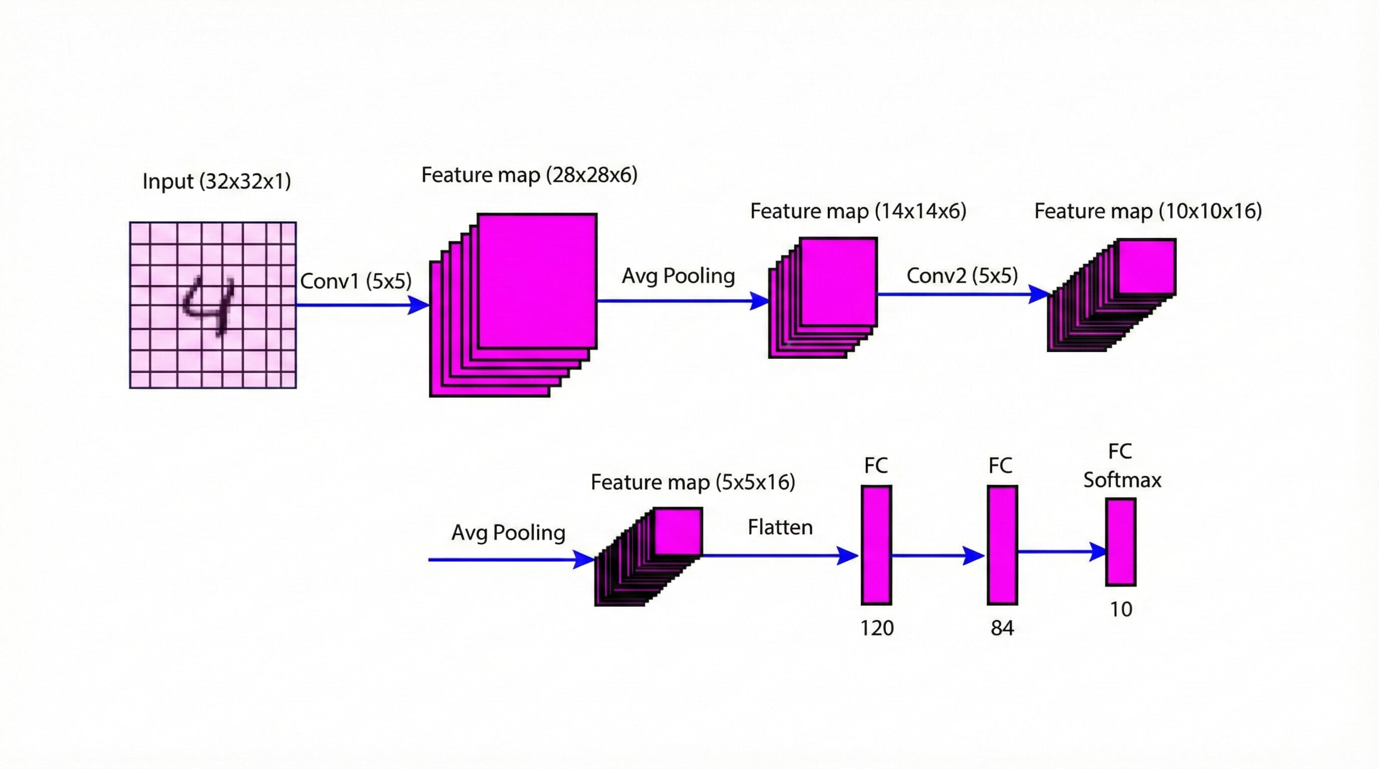
The LeNet5 network is made up of 2 convolutional layers, 2 average pooling layers, and 3 fully connected layers. We will teach you how to develop and train a convolutional neural network model based on LeNet5 architecture using Keras API. We will further evaluate the model performances on the test dataset.
If you are not aware of the LeNet architecture, then please read our previous blog post. By the end of this article, you will have a convolutional neural network model that can achieve an accuracy of over 99% on the MNIST dataset. Let’s dive right in!
Understanding The LeNet-5 architecture
LeNet5 is a convolutional neural network proposed by Yann LeCun and his research group in 1998 for recognizing handwritten and machine-printed characters. The LeNet5 network is a simple architecture with two convolutional layers, two average pooling layers, and three fully connected layers. The details of various layers are given in the figure and table below (Figure 1 and Table 1). You can go through our previous blog post.

Figure 1: LeNet-5 architecture overview
| Layer | Type | Input Size | Output Size | Activation Function | Kernel Size | Number of Filters | Number of Parameters |
|---|---|---|---|---|---|---|---|
| C1 | Convolutional | 32 x 32 x 1 | 28 x 28 x 6 | tanh | 5 x 5 | 6 | 156 |
| S1 | Average Pooling | 28 x 28 x 6 | 14 x 14 x 6 | tanh | 2 x 2 | - | 12 |
| C2 | Convolutional | 14 x 14 x 6 | 10 x 10 x 16 | tanh | 5 x 5 | 16 | 2,416 |
| S2 | Average Pooling | 10 x 10 x 16 | 5 x 5 x 16 | tanh | 2 x 2 | - | 32 |
| FC | Fully Connected | 5 x 5 x 16 | 1 x 1 x 120 | tanh | 4 x 4 | 120 | 19,320 |
| FC | Fully Connected | 1 x 1 x 120 | 1 x 1 x 84 | tanh | - | - | 10,164 |
| Output | Softmax | 1 x 1 x 84 | 1 x 1 x 10 | softmax | - | - | 850 |
Table 1: LeNet-5 layer-wise architecture summary
Practical Implementation
Here, the aim is to develop a convolutional neural network model similar to LeNet5 architecture to classify the MNIST dataset. You can find the source code here: LeNet5 Model.
Import Necessary Libraries
import keras
import keras.utils
from keras import datasets, layers, models
from keras.models import Sequential
from keras.layers import Conv2D, AveragePooling2D, MaxPooling2D, Flatten, Dense, Activation
import matplotlib.pyplot as plt
Load Dataset
Here, we will load the MNIST dataset and store it in the variables.
(x_train, y_train), (x_test, y_test) = datasets.mnist.load_data()Visualize The Data
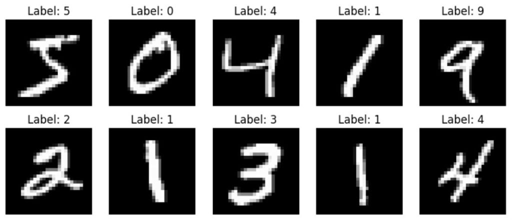
We can visualize the training data using the following code snippet.
plt.figure(figsize=(10, 4))  # Set The size Of The Figure
for i in range(10):
    plt.subplot(2, 5, i + 1)  # Make subplots for 10 images
    plt.imshow(x_train[i], cmap='gray')  # Display The grayscale images
    plt.title(f"Label: {y_train[i]}")  # Add labels
    plt.axis('off')  # Axis Labels Turned Off
plt.show()  # Displaying the plot
Figure 2: Sample MNIST images with their labels
Data Processing
Split The Data Into Training And Validation Set
Here, we will split the data into the training and validation set.
# Consider The First 50000 samples As The Training Dataset
x_train_main = x_train[:50000]
y_train_main = y_train[:50000]# Conside The Last 10000 Samples AS The Validation Dataset
x_val = x_train[50000:]
y_val = y_train[50000:]Normalize The Data
Normalize the pixel values of the image data by dividing them by 255. This will scale the pixel values within the range [0, 1].
x_train_main = x_train_main / 255.0
x_val=x_val/255.0
x_test = x_test / 255.0
Reshape data
Change the shape of the arrays to include the color channel of the images. Since the images are grayscale, the color channel is 1.
x_train_main = x_train_main.reshape(50000, 28, 28, 1)
x_val = x_val.reshape(10000, 28, 28, 1)
x_test = x_test.reshape(10000, 28, 28, 1)
One Hot Encoding
Perform one-hot encoding to convert categorical data into binary vectors. Each element in the binary vector corresponds to a class, and only one element is 1, while the rest are 0. For example, if there are 10 classes and the label is 3, the one-hot encoded vector would be [0, 0, 0, 1, 0, 0, 0, 0, 0, 0].
y_train_main = keras.utils.to_categorical(y_train_main, 10)
y_val = keras.utils.to_categorical(y_val, 10)
y_test = keras.utils.to_categorical(y_test, 10)
Build LeNet5 Model
#Create An Instance of Sequential Class.
LeNet5_Model=Sequential()# Add First Convolutional Layer
LeNet5_Model.add(Conv2D(6, kernel_size=(5, 5), activation='tanh', input_shape=(28, 28, 1)))# Add First Average Pooling Layer
LeNet5_Model.add(AveragePooling2D((2, 2)))# Add Second Convolutional Layer
LeNet5_Model.add(Conv2D(16, kernel_size=(5, 5), activation='tanh'))# Add Second Average Pooling Layer
LeNet5_Model.add(AveragePooling2D((2, 2)))# Flatten The Layer
LeNet5_Model.add(Flatten())# Add Dense Layer
LeNet5_Model.add(Dense(120, activation='tanh'))
LeNet5_Model.add(Dense(84, activation='tanh'))
LeNet5_Model.add(Dense(10, activation='softmax'))Compile The Model
LeNet5_Model.compile(loss='categorical_crossentropy', optimizer='adam', metrics=['accuracy'])Check Model Summary
LeNet5_Model.summary()Output: Model: "sequential"
_________________________________________________________________
Layer (type) Output Shape Param #
=================================================================
conv2d (Conv2D) (None, 24, 24, 6) 156
average_pooling2d (Average (None, 12, 12, 6) 0
Pooling2D)
conv2d_1 (Conv2D) (None, 8, 8, 16) 2416
average_pooling2d_1 (Avera (None, 4, 4, 16) 0
gePooling2D)
flatten (Flatten) (None, 256) 0
dense (Dense) (None, 120) 30840
dense_1 (Dense) (None, 84) 10164
dense_2 (Dense) (None, 10) 850
=================================================================
Total params: 44426 (173.54 KB)
Trainable params: 44426 (173.54 KB)
Non-trainable params: 0 (0.00 Byte)Train The Model
LeNet5_Model.fit(x_train_main, y_train_main, epochs=20, batch_size=128, validation_data=(x_val, y_val))Epoch 1/20
391/391 [==============================] - 23s 54ms/step - loss: 0.4121 - accuracy: 0.8783 - val_loss: 0.1799 - val_accuracy: 0.9485
Epoch 2/20
391/391 [==============================] - 19s 49ms/step - loss: 0.1448 - accuracy: 0.9569 - val_loss: 0.1098 - val_accuracy: 0.9675
Epoch 3/20
391/391 [==============================] - 19s 49ms/step - loss: 0.0908 - accuracy: 0.9726 - val_loss: 0.0801 - val_accuracy: 0.9757
Epoch 4/20
391/391 [==============================] - 21s 54ms/step - loss: 0.0668 - accuracy: 0.9800 - val_loss: 0.0689 - val_accuracy: 0.9790
Epoch 5/20
391/391 [==============================] - 19s 49ms/step - loss: 0.0525 - accuracy: 0.9839 - val_loss: 0.0604 - val_accuracy: 0.9821
Epoch 6/20
391/391 [==============================] - 23s 59ms/step - loss: 0.0453 - accuracy: 0.9860 - val_loss: 0.0580 - val_accuracy: 0.9827
Epoch 7/20
391/391 [==============================] - 22s 56ms/step - loss: 0.0368 - accuracy: 0.9890 - val_loss: 0.0558 - val_accuracy: 0.9831
Epoch 8/20
391/391 [==============================] - 21s 53ms/step - loss: 0.0313 - accuracy: 0.9900 - val_loss: 0.0475 - val_accuracy: 0.9867
Epoch 9/20
391/391 [==============================] - 19s 49ms/step - loss: 0.0270 - accuracy: 0.9915 - val_loss: 0.0518 - val_accuracy: 0.9848
Epoch 10/20
391/391 [==============================] - 21s 53ms/step - loss: 0.0223 - accuracy: 0.9933 - val_loss: 0.0572 - val_accuracy: 0.9840
Epoch 11/20
391/391 [==============================] - 19s 50ms/step - loss: 0.0198 - accuracy: 0.9939 - val_loss: 0.0469 - val_accuracy: 0.9862
Epoch 12/20
391/391 [==============================] - 19s 49ms/step - loss: 0.0162 - accuracy: 0.9953 - val_loss: 0.0578 - val_accuracy: 0.9835
Epoch 13/20
391/391 [==============================] - 21s 53ms/step - loss: 0.0142 - accuracy: 0.9958 - val_loss: 0.0514 - val_accuracy: 0.9866
Epoch 14/20
391/391 [==============================] - 19s 49ms/step - loss: 0.0121 - accuracy: 0.9962 - val_loss: 0.0506 - val_accuracy: 0.9853
Epoch 15/20
391/391 [==============================] - 21s 55ms/step - loss: 0.0111 - accuracy: 0.9967 - val_loss: 0.0600 - val_accuracy: 0.9853
Epoch 16/20
391/391 [==============================] - 19s 49ms/step - loss: 0.0096 - accuracy: 0.9970 - val_loss: 0.0534 - val_accuracy: 0.9845
Epoch 17/20
391/391 [==============================] - 23s 58ms/step - loss: 0.0093 - accuracy: 0.9973 - val_loss: 0.0553 - val_accuracy: 0.9851
Epoch 18/20
391/391 [==============================] - 19s 49ms/step - loss: 0.0082 - accuracy: 0.9976 - val_loss: 0.0516 - val_accuracy: 0.9867
Epoch 19/20
391/391 [==============================] - 19s 49ms/step - loss: 0.0053 - accuracy: 0.9986 - val_loss: 0.0539 - val_accuracy: 0.9859
Epoch 20/20
391/391 [==============================] - 21s 54ms/step - loss: 0.0058 - accuracy: 0.9983 - val_loss: 0.0536 - val_accuracy: 0.9856Evaluate The Model Performance On The Test Dataset
test_loss, test_acc = LeNet5_Model.evaluate(x_test, y_test)
print('Test accuracy:', test_acc)Output:
313/313 [==============================] - 1s 4ms/step - loss: 0.0496 - accuracy: 0.9853
Test accuracy: 0.9853000044822693Conclusion
In this article, we learned how to develop a convolutional neural network based on LeNet5 architecture using Keras. We found that the performance of the model in classifying fashion in the MNIST dataset is more than 98%.
We hope you enjoyed this article and learned something new. If you have any questions or feedback, please leave a comment below. Thank you for reading!
Frequently Asked Questions
How many layers are in LeNet5?
LeNet5 is a pioneering convolutional neural network architecture that was designed to recognize handwritten digits. It has seven layers, excluding the input layer. The layers are two convolutional layers, two subsampling (pooling) layers, and three fully connected layers, ending in a softmax output layer.
Was LeNet the first CNN?
Lenet5, developed by Yann LeCun and his research group in the late 1880s, was one of the earliest and most influential convolutional neural networks. Although it was not the very first CNN, the development of LeNet5 laid the groundwork for modern deep learning and computer vision applications.

