Overview
Would you like to visit a website that displays images of people who don’t exist in real life? If so, then check this website and see what happens. You will notice that it loads new faces every time you refresh the page. However, these faces are not real; they are entirely artificially generated. This may seem like magic, but the generative adversarial networks (GANs) let this magic happen in the background.
Generative Adversarial Networks (GANs) are an AI framework that has revolutionized how machines understand and generate content. It was proposed by Ian J. Goodfellow, along with his co-authors, in 2014. Yann LeCun, a pioneering figure in deep learning and artificial intelligence, called GANs “the most interesting idea in the last ten years in machine learning”.
In this article, you will learn the basics of GANs and how to develop a GAN model using Keras and TensorFlow in Python. The model will generate a dataset similar to the MNIST dataset, a collection of handwritten digits. Let’s explore GANs together on this exciting journey.
Understanding the Mechanics of GANs Through Analogies
We can better understand the GANs with the help of a real-life example where a cricket batter is trying to learn how to play leg spin bowling.
Leg-spin bowling is a particular type of bowling known for its deceptive flight and spin, making it difficult for batsmen to predict the ball’s trajectory. Let’s assume that the cricket batter is the generator, whereas the leg-spin bowler is the discriminator.
The Cricket Batter (Generator)
Imagine that the batter is struggling to play against leg-spin bowling. The batter aims to improve and become proficient at facing leg-spin deliveries.
The Leg-spin Bowler (Discriminator)
Now imagine that we have a skilled leg-spin bowler who can confuse batters with variations in flight, spin, and pace. The objective of the leg-spin bowler is to deceive the batsman by exploiting his weakness in playing leg-spin.
The Learning Process
Consider a situation where the batter and leg-spin bowler started playing. Initially, the batsman may find it challenging to play leg spin, which can often lead to mistimed shots or misjudgments, causing him to get out quickly.
However, with each delivery, the batter learns from his mistakes. He closely observes the bowler’s grips, the number of revolutions on the ball, or any other subtle signs that may indicate the type of delivery. Based on the observation, the batsman adjusts his footwork, timing, and shot selection. With time, the batsman becomes more confident and capable of playing leg-spin bowling.
As the batter improves his skills, the leg-spin bowler must also modify his strategy by closely observing the batter’s weakness and making necessary changes in his bowling tactics. For example, the leg-spin bower may introduce new variations in his bowling, such as altering bowling angles, using googlies, flippers, carrom balls, or better disguising his deliveries.
Ultimately, the aim of the batter (the generator) is to become an expert in dealing with leg-spin deliveries, while the objective of the leg-spin bowler is to improve his skills in deceiving the batsman.
The dynamics between the cricket batter and leg-spin bowler depicted above reflect the adversarial training process in the GANs where both the generator (the cricket batter) and discriminator (the leg-spinner) try to improve continuously through competition and adaptation. In the section below, we will try to understand the architecture of GANs.
Architecture Of The Generative Adversarial Network
The architecture of GANs consists of two neural networks: a generator and a discriminator. Here, we will discuss them one by one:
Generator
The generator starts with random noises as input, usually drawn from a simple distribution such as the Gaussian distribution. The input noise passes through multiple layers in a neural network. Mathematical operations are performed in each layer, gradually shaping the input into a meaningful output that ideally resembles the real data samples.
The main objective of the generator is to deceive the discriminator into believing that the generated outputs (also termed as the fake outputs) are authentic by producing them similar to the real data samples.
Discriminator
The discriminator is a binary classification model whose primary task is to accurately distinguish the two categories: real data and fake data. In the discriminator model, the inputs are fake data produced by the generator and the real data of the training dataset.
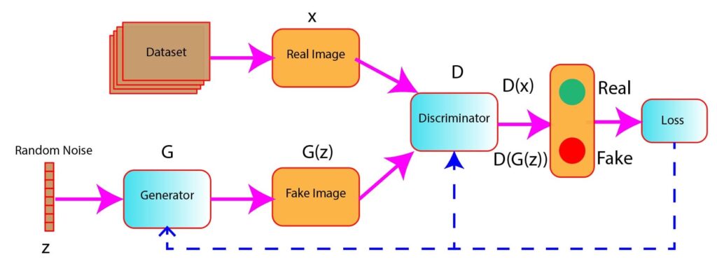
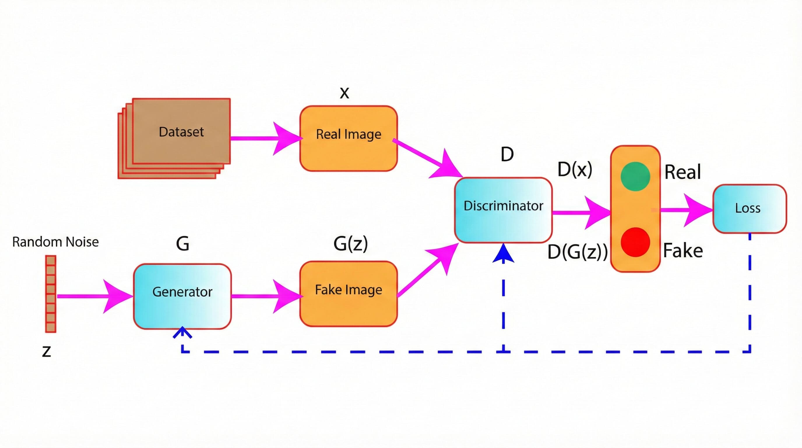
Figure 1: Architecture of GANs (generator and discriminator)
Visualize The Interaction between Generator And Discriminator
-
As shown in Figure 1, a random noise z acts as an input in the generator model. The generator generates fake images G(z) from the random noise.
-
The fake images G(z), along with real images (x), are fed into the discriminator model D.
-
In the next step, the discriminator classifies the images, whether real or fake.
-
Based on the prediction of the discrimination, the loss is computed, and this loss is used to update the weights of the Generator and the Discriminator using backpropagation.
Practical Implementation
In the previous sections, we learned the general architecture of GANs and how they work with the help of an analogy. Here, we will develop a generative adversarial network to generate an image similar to the MNIST dataset. We will use TensorFlow and Keras to implement the GANs architecture, training it to produce realistic handwritten digits. We will implement the code step-by-step, explaining each component as we progress. Also, please click the link to open the code in Google colaboratory.
Import Dependencies
import tensorflow as tf
from tensorflow.keras import layers, models
import numpy as np
import matplotlib.pyplot as plt
Load And Process Dataset
Load the training images from the MNIST dataset.
(train_images, _), (_, _) =tf.keras.datasets.mnist.load_data()print(train_images.shape)output:
(60000, 28, 28)# Visualize The First Few Images From The Dataset
plt.figure(figsize=(10, 10))
for i in range(25):
plt.subplot(5, 5, i + 1)
plt.imshow(train_images[i], cmap='gray')
plt.axis('off')
plt.show()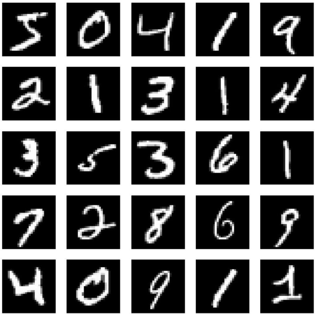
Figure 2: First few images from the MNIST dataset
The line of code below reshapes the training images to have dimensions suitable for input into a convolutional neural network (CNN). It does that by adding a single channel dimension (for grayscale images) and converting the data type to float32.
# Reshape The Data
train_images = train_images.reshape(train_images.shape[0], 28, 28, 1).astype('float32')# Normalize The Data Within The Range [-1, 1]
train_images = (train_images - 127.5) / 127.5print(train_images.shape)Output:
(60000, 28, 28, 1)Define Generator Model
-
The generator model started with a dense layer that takes the random noise as input, and the resulting output shape is (7, 7, 256).
-
Data is further normalized using BatchNormalization() and followed by LeakyReLU() activation layer to introduce non-linearity to the data.
-
There are several convolutional transpose layers to upsample the tensor, which gradually increases the spatial dimensions while reducing depth. The objective is to achieve the output shape of (28, 28, 1), matching the format of the MNIST dataset.
def make_generator_model():
  model=models.Sequential()
  model.add(layers.Dense(7*7*256, use_bias=False, input_shape=(100,)))
  model.add(layers.BatchNormalization())
  model.add(layers.LeakyReLU())
  model.add(layers.Reshape((7, 7, 256)))
  assert model.output_shape == (None, 7, 7, 256)

  model.add(layers.Conv2DTranspose(filters=128, kernel_size=(5, 5), strides=(1, 1), padding='same', use_bias=False))
  assert model.output_shape == (None, 7, 7, 128)
  model.add(layers.BatchNormalization())
  model.add(layers.LeakyReLU())

  model.add(layers.Conv2DTranspose(filters=64, kernel_size=(5, 5), strides=(2, 2), padding='same', use_bias=False))
  assert model.output_shape == (None, 14, 14, 64)
  model.add(layers.BatchNormalization())
  model.add(layers.LeakyReLU())

  model.add(layers.Conv2DTranspose(filters=1, kernel_size=(5, 5), strides=(2, 2), padding='same', use_bias=False, activation='tanh'))
  assert model.output_shape == (None, 28, 28, 1)

return modelgenerator = make_generator_model()generator.summary()Model: "sequential_4"
_________________________________________________________________
Layer (type) Output Shape Param #
=================================================================
dense_4 (Dense) (None, 12544) 1254400
batch_normalization_6 (Bat (None, 12544) 50176
chNormalization)
leaky_re_lu_10 (LeakyReLU) (None, 12544) 0
reshape_2 (Reshape) (None, 7, 7, 256) 0
conv2d_transpose_6 (Conv2D (None, 7, 7, 128) 819200
Transpose)
batch_normalization_7 (Bat (None, 7, 7, 128) 512
chNormalization)
leaky_re_lu_11 (LeakyReLU) (None, 7, 7, 128) 0
conv2d_transpose_7 (Conv2D (None, 14, 14, 64) 204800
Transpose)
batch_normalization_8 (Bat (None, 14, 14, 64) 256
chNormalization)
leaky_re_lu_12 (LeakyReLU) (None, 14, 14, 64) 0
conv2d_transpose_8 (Conv2D (None, 28, 28, 1) 1600
Transpose)
=================================================================
Total params: 2330944 (8.89 MB)
Trainable params: 2305472 (8.79 MB)
Non-trainable params: 25472 (99.50 KB)
_________________________________________________________________Define Discriminator Model
-
In the code below, two convolutional layers extract features using filters and downsampling.
-
ReLu activation function introduces non-linearity followed by dropout regularization to prevent overfitting.
-
Finally, add a dense layer. As we can see, there is only one neuron in the dense layer, and it is because the task of the discriminator is binary classification, determining whether an input image is real or fake.
def make_discriminator_model():
    model = models.Sequential()
    model.add(layers.Conv2D(filters=64, kernel_size=(5, 5), strides=(2, 2), padding='same', input_shape=[28, 28, 1]))
    model.add(layers.LeakyReLU())
    model.add(layers.Dropout(0.3))

    model.add(layers.Conv2D(filters=128, kernel_size=(5, 5), strides=(2, 2), padding='same'))
    model.add(layers.LeakyReLU())
    model.add(layers.Dropout(0.3))

    model.add(layers.Flatten())
    model.add(layers.Dense(1))

return modeldiscriminator = make_discriminator_model()discriminator.summary()Model: "sequential_5"
_________________________________________________________________
Layer (type) Output Shape Param #
=================================================================
conv2d_4 (Conv2D) (None, 14, 14, 64) 1664
leaky_re_lu_13 (LeakyReLU) (None, 14, 14, 64) 0
dropout_4 (Dropout) (None, 14, 14, 64) 0
conv2d_5 (Conv2D) (None, 7, 7, 128) 204928
leaky_re_lu_14 (LeakyReLU) (None, 7, 7, 128) 0
dropout_5 (Dropout) (None, 7, 7, 128) 0
flatten_2 (Flatten) (None, 6272) 0
dense_5 (Dense) (None, 1) 6273
=================================================================
Total params: 212865 (831.50 KB)
Trainable params: 212865 (831.50 KB)
Non-trainable params: 0 (0.00 Byte)
_________________________________________________________________Define Loss And Optimizer
# Define The Loss Functions
cross_entropy = tf.keras.losses.BinaryCrossentropy(from_logits=True)
The code below computes two types of discriminator losses:
-
real_loss: It measures how well the discriminator correctly identifies real data as real
-
fake_loss: It measures how well the discriminator correctly identifies fake/generated data as fake.
# Define The Discriminator Loss
def discriminator_loss(real_output, fake_output):
    real_loss = cross_entropy(tf.ones_like(real_output), real_output)
    fake_loss = cross_entropy(tf.zeros_like(fake_output), fake_output)
    total_loss = real_loss + fake_loss
    return total_loss
In the code below, the generator loss measures how well the generator can produce fake data that resembles real data.
# Define The Generator Loss
def generator_loss(fake_output):
return cross_entropy(tf.ones_like(fake_output), fake_output)# Deine Optimizer
generator_optimizer = tf.keras.optimizers.Adam(learning_rate=1e-4)
discriminator_optimizer = tf.keras.optimizers.Adam(learning_rate=1e-4)Define Training Step
# Create the generator and discriminator
generator = make_generator_model()
discriminator = make_discriminator_model()
Implement a training step where the generator and discriminator are updated based on the computed losses.
# Define The Training Step
@tf.function
def train_step(images):
  noise = tf.random.normal([BATCH_SIZE, NOISE_DIM])   # Generate Noise Sample
  with tf.GradientTape() as gen_tape, tf.GradientTape() as disc_tape:
    generated_images = generator(noise, training=True)  # Execute The Generator While Using The Noise As Input

    real_output = discriminator(images, training=True)     # Execute The Discriminator Using Real Imnage As Input
    fake_output = discriminator(generated_images, training=True) # Execute The Discriminator Using Fake Image As Input

    disc_loss = discriminator_loss(real_output, fake_output)   # Compute The Discriminator Loss
    gen_loss = generator_loss(fake_output)                     # Compute The Generator Loss

  gradients_of_generator = gen_tape.gradient(gen_loss, generator.trainable_variables)  # Compute The Gradient Of The Generator With Respect To Trainable Parameters
  gradients_of_discriminator = disc_tape.gradient(disc_loss, discriminator.trainable_variables)  # Compute The Gradient Of The Discriminator With Respect To Trainable Parameters

  generator_optimizer.apply_gradients(zip(gradients_of_generator, generator.trainable_variables))  # Apply The Computed Gradient To Update The Parameters Of The Generator Using Gradient Optimizer
  discriminator_optimizer.apply_gradients(zip(gradients_of_discriminator, discriminator.trainable_variables))  # Apply The Computed Gradient To Update The Parameters Of The Discriminator Using Gradient Optimizer

  return gen_loss, disc_loss
Train The Model
# Define Parameters
EPOCHS = 25
NOISE_DIM = 100
BATCH_SIZE = 128# Define Function To Generate And Save Images
def generate_and_save_images(model, epoch, test_input):
predictions = model(test_input, training=False)
fig = plt.figure(figsize=(10, 10))
for i in range(predictions.shape[0]):
plt.subplot(4, 4, i+1)
plt.imshow(predictions[i, :, :, 0] * 127.5 + 127.5, cmap='gray')
plt.axis('off')
plt.savefig('image_at_epoch_{:04d}.png'.format(epoch))
plt.show()# Training Loop
generator_losses = []
discriminator_losses = []
def train(dataset, epochs):
for epoch in range(epochs):
print(epoch)
for batch in dataset:
gen_loss, disc_loss = train_step(batch)
generator_losses.append(gen_loss)
discriminator_losses.append(disc_loss)
# Produce images for the GIF as we go
print(f'Epoch {epoch+1}, Generator Loss: {gen_loss}, Discriminator Loss: {disc_loss}')
if (epoch + 1) % 10 == 0:
generate_and_save_images(generator, epoch, seed)# Train Model
# Create batches of the dataset
train_dataset = tf.data.Dataset.from_tensor_slices(train_images).shuffle(60000).batch(BATCH_SIZE)
# Generate seed to visualize progress
seed = tf.random.normal([16, NOISE_DIM])
# Train the model
train(train_dataset, EPOCHS)Output:
Epoch 1, Generator Loss: 0.9692994356155396, Discriminator Loss: 1.0385773181915283
Epoch 2, Generator Loss: 0.7986713647842407, Discriminator Loss: 1.4925286769866943
Epoch 3, Generator Loss: 0.7524862289428711, Discriminator Loss: 1.4109594821929932
Epoch 4, Generator Loss: 1.027969241142273, Discriminator Loss: 1.0305981636047363
Epoch 5, Generator Loss: 0.9398350119590759, Discriminator Loss: 1.1616337299346924
Epoch 6, Generator Loss: 0.8576270341873169, Discriminator Loss: 1.2590687274932861
Epoch 7, Generator Loss: 1.0282213687896729, Discriminator Loss: 1.1530981063842773
Epoch 8, Generator Loss: 1.2133488655090332, Discriminator Loss: 1.0967073440551758
Epoch 9, Generator Loss: 1.0876505374908447, Discriminator Loss: 1.1350641250610352
Epoch 10, Generator Loss: 1.0201687812805176, Discriminator Loss: 1.1206631660461426The image below shows the generated images after 300 epochs (Figure 3). What do you think about the generated images below? Are they similar to the MNIST dataset? Do we need further improvement?
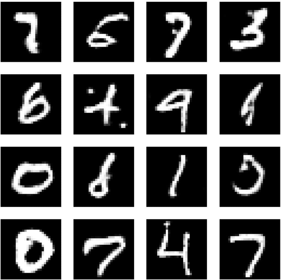
Figure 3: Generated images after training (around 300 epochs)
Visualize The Losses
Use the following code snippet to compute the average losses over epochs.
# Calculate the number of batches in your dataset
num_batches = len(generator_losses) // batch_size

# Calculate average losses over epochs
average_generator_losses = [np.mean(generator_losses[i:i+num_batches]) for i in range(0, len(generator_losses), num_batches)]
average_discriminator_losses = [np.mean(discriminator_losses[i:i+num_batches]) for i in range(0, len(discriminator_losses), num_batches)]
Now plot the average losses.
# Plot average losses
plt.plot(average_generator_losses, label='Generator Loss')
plt.plot(average_discriminator_losses, label='Discriminator Loss')
plt.xlabel('Epoch')
plt.ylabel('Loss')
plt.title('Generator and Discriminator Losses (Smoothed)')
plt.legend()
plt.show()
The figure below shows that the generator losses increase initially (during the first few epochs) (Figure 4). This indicates that the generator is struggling to produce high-quality fake images to deceive the discriminator. However, as the training progresses, the generator losses steadily decrease and eventually stabilize. This indicates that the generator is progressively improving at fooling the discriminator by generating images that resemble real images.
Conversely, the discriminator losses decrease initially (within the first few epochs). This indicates that the discriminator quickly becomes efficient at distinguishing between real and fake images. However, as training advances, the discriminator losses increase gradually and stabilize. This implies that the discriminator faces increasing difficulty in identifying fake images as fake, possibly due to the generator producing more realistic fake images.
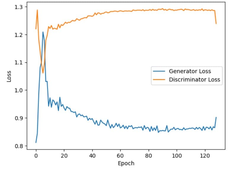
Figure 4: Generator and discriminator losses during training
Conclusions
In this blog post, we learned the fundamental concepts of GANs involving two neural networks (a generator and a discriminator) competing with each other to generate synthetic data that is indistinguishable from real data.
We also developed a GAN model using TensorFlow and Keras to generate images similar to the MNIST dataset. We observe that the generated images are identical to the real MNIST dataset, showcasing the power of GANs in generating realistic data.
However, it is essential to remember that GANs have their challenges, like all other machine learning models. Training GANs require precise adjustments to model parameters and training methods, making it complex and time-consuming. However, with patience and persistence, the rewards can be great.
The potential of GANS is vast and exciting potential for the future. We can use GANs to generate art and music, simulate realistic video game environments, and advance scientific research, among other things.
In this article, we provided the theoretical details of GANs very briefly. If you wish to know more details, you can visit our previous article on GANs.
Frequently Asked Questions
How do GANs work?
There are two neural networks in GANs: the generator and the discriminator. The task of the generator is to create fake data that are similar to the real data. The task of the discriminator is to check if the data is real or fake. These two networks are trained simultaneously in a game-like scenario where the aim of the generator is to fool the discriminator. As training progresses, the generator gets better at producing realistic data, while the discriminator gets better at identifying fake data.
Why are GANs difficult to train?
Training generative adversarial networks (GANS) requires a delicate balance between the generator and the discriminator. This makes GANs difficult to train. If one component outperforms the other, it may lead to instability and problems such as mode collapse. Moreover, the adversarial nature of GANs and the requirement for precise tuning of hyperparameters also add to the difficulty of training GANs.
Is GAN supervised or unsupervised?
Generative adversarial networks (GANs) are generally unsupervised learning algorithms. We can generate realistic data without the need for labeled data using GANs.
References
Architecture Of Generative Adversarial Networks
