Overview
Would you like to explore a website that displays images of people who don’t exist in real life? Go to this website and refresh the page. You will notice a new face will appear every time you refresh the page. However, these people do not exist in real life. Do you find it believable? Instead, the images are artificially generated using generative adversarial networks (GANs).
If you want to know the technology behind the GAN, then this article is for you. In this article, you will learn how the generative adversarial network works and a practical implementation of the network to generate images similar to the fashion MNIST dataset. We will use TensorFlow and Keras to develop a GAN model.
Understanding GAN with the help of an analogy
Let us try to understand GAN with the help of the analogy. Imagine a hypothetical scenario where two partners make fake currencies: a counterfeiter (generator) and a police officer (discriminator).
The job of the counterfeiter is to create fake currency indistinguishable from real currency. Conversely, the job of the police officer is to detect which currencies are authentic and which are fake. The process works as follows:
-
In the initial stage, the counterfeiter does not have sufficient knowledge to make fake currency. However, he started with his limited knowledge and made some fake currencies. He gave them to the police officer for evaluation.
-
The police officer quickly identifies the currencies as fake and gives the counterfeiter feedback on why those currencies are fake.
-
The counterfeiter learns from feedback given by the police officer and tries to correct his mistakes. This might involve using higher-quality materials, improving printing processes, and improving techniques to produce more convincing fake currency.
-
This iterative process continues with the counterfeiter continuously trying to improve methods to produce more convincing fake currency to evade the police officer.
-
In the meantime, the police officer also adapts and improves his ability to identify fake currencies. By analyzing fake currencies and identifying patterns and characteristics, he becomes more expert in differentiating them from authentic currencies.
This ongoing cycle of iteration and adaptation characterizes the dynamic interplay between the two parties (generator and discriminator) in a Generative Adversarial Network (GAN).
Architecture Of GAN
The GAN architecture comprises two neural networks: the generator and the discriminator.
Generator
Consider the figure below (Figure 1). As we can see, the generator takes random noise as input, which is usually drawn from simple distribution functions such as Gaussian distribution. The noise is passed through several layers in the generator consisting of densely connected layers, convolutional layers, or a combination of both.
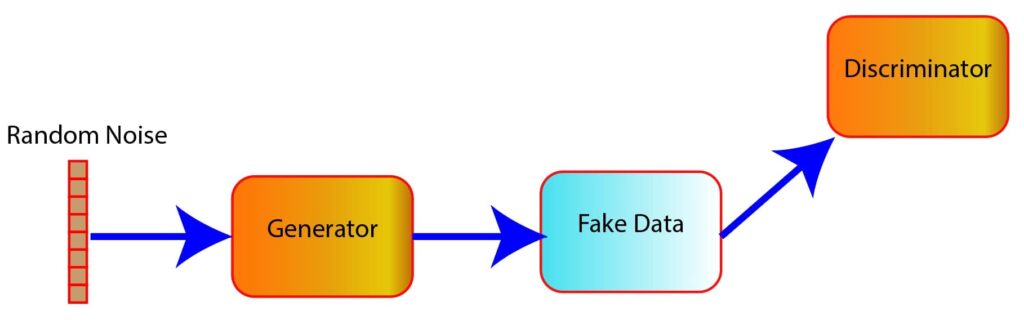
Figure 1: High-level view of how the generator works
Now, you might wonder what is happening inside the generator and how it creates fake data from random noise. Let us have a look at the following image to get a high-level overview of what is happening inside the generator network (Figure 2).
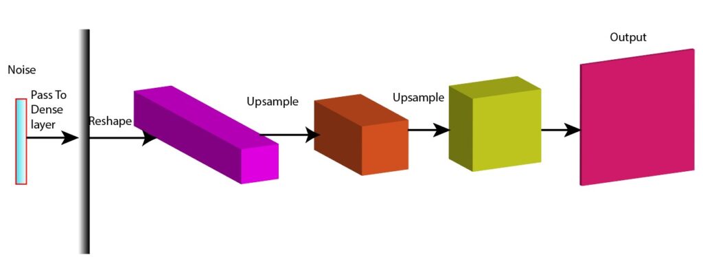
Figure 2: Inside the generator network (illustration)
-
On the left-hand side of the figure, we are using random noise (vertical multi-colored bar) as input to the network. This represents the initial data or signal that we want to process.
-
The noise is passed through a dense layer that transforms the data by applying weight and biases to produce a new representation.
-
The data is further reshaped, which makes the data suitable for the subsequent convolutional layer.
-
The reshaped data now enters a transposed convolutional layer that help detect patterns and features within the data and up-sampling the data.
-
The unsampled data is further passed through another transposed convolutional layer. The shape of the output from the transposed convolutional layer should be the same as the shape of real data.
Discriminator
The main objective of the discriminator is to accurately differentiate between the two categories: real data and fake data. A discriminator network takes both the fake data (generated by the generator) and real data as input, performs binary classification and assigns a label to each sample.
Let us assume that we want to train a GAN to generate realistic images of cats. In that case, the real data are the actual images of cats, and fake data are the images generated by the generator. The discriminator network will label real data of the training dataset as 1 and fake data generated by the generator as 0.
The figure below will help us to understand the discriminator network (Figure 3).
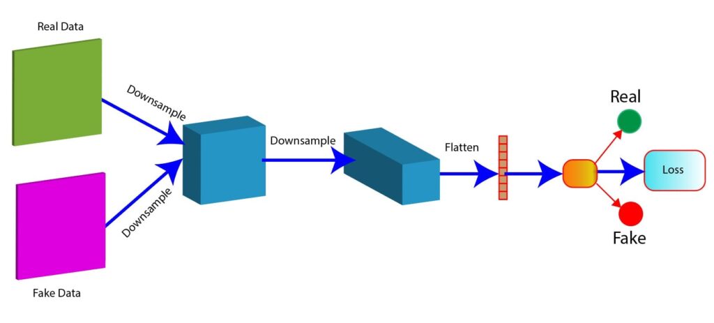
Figure 3: Discriminator network (illustration)
-
In the figure, there are two types of data: real data and fake data. Both the data samples serve as input to the discriminator network.
-
We then downsample the data that involves convolutions or max-pooling to reduce the spatial dimension of the data. As we can see in the figure, the data are downsampled twice.
-
After the convolutional layers, a flattened layer converts 2D feature maps into a 1D vector. This prepares the data for fully connected layers.
-
Then, we compute a loss function, which helps to evaluate how well it distinguishes real from fake data.
-
The output of the discriminator is a probability score. The score should be close to 1 for real data, and for fake data, the score should be close to 0.
Understand The Interaction Between the Generator And Discriminator
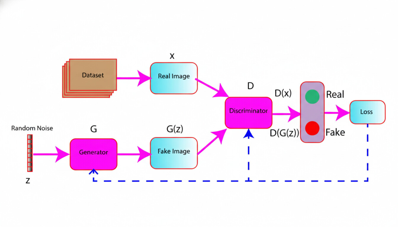
The figure below shows a high-level overview of the learning process of the GAN involving generator and discriminator network (Figure 4).
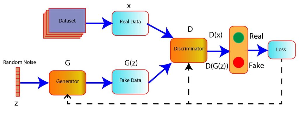
Figure 4: High-level GAN training loop (generator–discriminator interaction)
-
In the figure, a random noise z is passed as input in the generator model. The generator generates fake data G(z) from the random noise.
-
In the discriminator model, the inputs are the fake data G(z) and real images (x).
-
The task of the discriminator is to classify the data, whether real or fake.
-
The loss is computed based on the prediction of the discriminator. This loss is used further to update the weights of the generator and discriminator using backpropagation.
Practical Implementation
In this section, we will develop a GAN model to generate images similar to the fashion MNIST dataset. We will use Tensorflow and Keras in Python to construct and train our model. Let’s begin the journey.
Import Necessary Libraries
import tensorflow as tf
from tensorflow.keras import layers, models
import numpy as np
import matplotlib.pyplot as plt
Load And Process The Fashion MNIST Dataset
# Load The Dataset
fashion_mnist = tf.keras.datasets.fashion_mnist
(train_img, _), (_, _) = fashion_mnist.load_data()# Visualize The First Few Images
plt.figure(figsize=(10,10))
for i in range(25):
plt.subplot(5,5,i+1)
plt.xticks([])
plt.yticks([])
plt.grid(False)
plt.imshow(train_img[i], cmap=plt.cm.binary)
plt.show()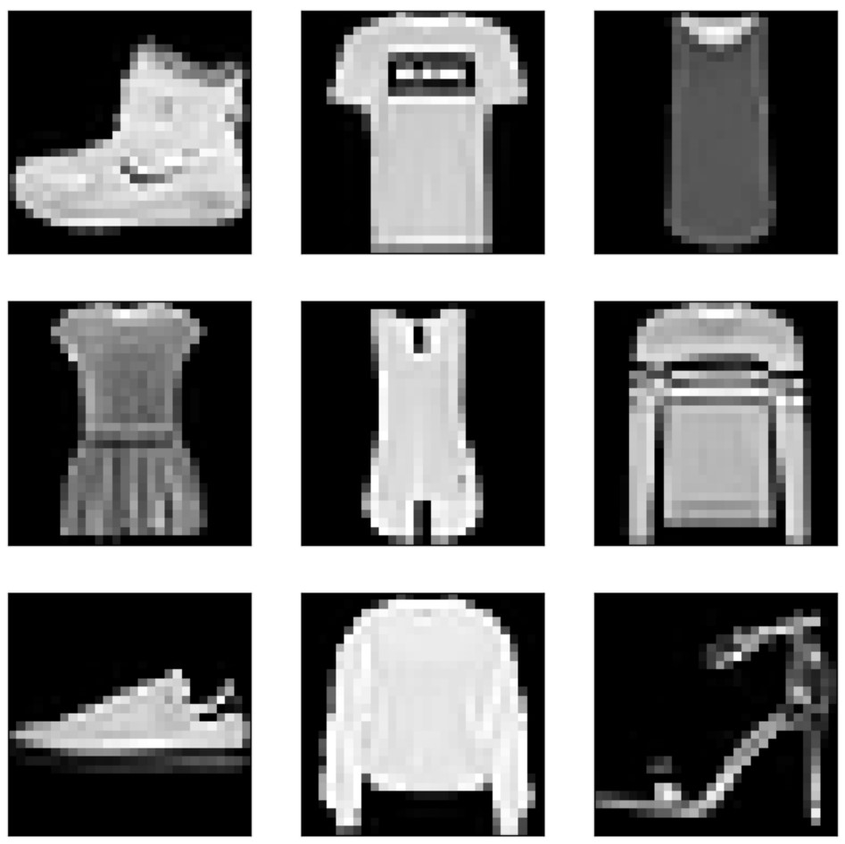
Figure 5: Sample images from the Fashion MNIST dataset
print(train_img.shape)The following line of code will reshape the training images to have dimensions suitable for input into a convolutional neural network (CNN). To make that happen, we add a single channel dimension (for grayscale images) and convert the data type to float32.
# Reshape The Data
train_img = train_img.reshape(train_img.shape[0], 28, 28, 1).astype('float32')# Normalize The Data Within The range[-1, 1]
train_img = (train_img - 127.5) / 127.5 # Normalize to [-1, 1]Define Generator Model
The code below starts with a dense layer that transforms a 100-dimensional input into a 7x7x512 tensor. It then progressively upsamples the tensors through a series of transposed convolutional layers with batch normalization and LeakyReLU activations. The shape of the output is a 28×28 single-channel image.
def create_generator_model():
    net = models.Sequential()
    # Add A Dense Layer With Input Shape of (100, )And Output Shape Of 7*7*512 units
    net.add(layers.Dense(7*7*512, use_bias=False, input_shape=(100,)))
    net.add(layers.BatchNormalization())
    net.add(layers.LeakyReLU())

    net.add(layers.Reshape((7, 7, 512)))
    assert net.output_shape == (None, 7, 7, 512)

    # Add A Transposed Convolutional Layer
    net.add(layers.Conv2DTranspose(filters=128, kernel_size=(5, 5), strides=(1, 1), padding='same', use_bias=False))
    assert net.output_shape == (None, 7, 7, 128)
    net.add(layers.BatchNormalization())
    net.add(layers.LeakyReLU())

    # Add A Transposed Convolutional Layer
    net.add(layers.Conv2DTranspose(filters=64, kernel_size=(5, 5), strides=(2, 2), padding='same', use_bias=False))
    assert net.output_shape == (None, 14, 14, 64)
    net.add(layers.BatchNormalization())
    net.add(layers.LeakyReLU())

    # Add A Transposed Convolutional Layer
    net.add(layers.Conv2DTranspose(filters=1, kernel_size=(5, 5), strides=(2, 2), padding='same', use_bias=False, activation='tanh'))
    assert net.output_shape == (None, 28, 28, 1)

return netgenerator = create_generator_model()We can view the details of the generator network using the following code snippet.
generator.summary()Output:
Model: "sequential"
_________________________________________________________________
Layer (type) Output Shape Param #
=================================================================
dense (Dense) (None, 25088) 2508800
batch_normalization (Batch (None, 25088) 100352
Normalization)
leaky_re_lu (LeakyReLU) (None, 25088) 0
reshape (Reshape) (None, 7, 7, 512) 0
conv2d_transpose (Conv2DTr (None, 7, 7, 128) 1638400
anspose)
batch_normalization_1 (Bat (None, 7, 7, 128) 512
chNormalization)
leaky_re_lu_1 (LeakyReLU) (None, 7, 7, 128) 0
conv2d_transpose_1 (Conv2D (None, 14, 14, 64) 204800
Transpose)
batch_normalization_2 (Bat (None, 14, 14, 64) 256
chNormalization)
leaky_re_lu_2 (LeakyReLU) (None, 14, 14, 64) 0
conv2d_transpose_2 (Conv2D (None, 28, 28, 1) 1600
Transpose)
=================================================================
Total params: 4454720 (16.99 MB)
Trainable params: 4404160 (16.80 MB)
Non-trainable params: 50560 (197.50 KB)
_________________________________________________________________Define Discriminator Model
Here, we construct a neural network composed of two convolutional layers, each followed by a LeakyReLU activation and ** dropout**for regularization, and ends with a dense layer to output a single value.
def Create_discriminator_model():
    # Initialize A Sequential Model
    net = models.Sequential()

    # Add A Convolutional Layer
    net.add(layers.Conv2D(filters=64, kernel_size=(5, 5), strides=(2, 2), padding='same', input_shape=[28, 28, 1]))
    net.add(layers.LeakyReLU())
    net.add(layers.Dropout(0.3))

    # Add A Convolutional Layer
    net.add(layers.Conv2D(filters=128, kernel_size=(5, 5), strides=(2, 2), padding='same'))
    net.add(layers.LeakyReLU())
    net.add(layers.Dropout(0.3))

    # Flatten The Output
    net.add(layers.Flatten())
    # Dense Layer With 1 Unit
    net.add(layers.Dense(1))

return netdiscriminator = Create_discriminator_model()We can view the details of the discriminator network by using the code below.
discriminator.summary()Output:
________________________________________________________________
Layer (type) Output Shape Param #
=================================================================
conv2d (Conv2D) (None, 14, 14, 64) 1664
leaky_re_lu_3 (LeakyReLU) (None, 14, 14, 64) 0
dropout (Dropout) (None, 14, 14, 64) 0
conv2d_1 (Conv2D) (None, 7, 7, 128) 204928
leaky_re_lu_4 (LeakyReLU) (None, 7, 7, 128) 0
dropout_1 (Dropout) (None, 7, 7, 128) 0
flatten (Flatten) (None, 6272) 0
dense_1 (Dense) (None, 1) 6273
=================================================================
Total params: 212865 (831.50 KB)
Trainable params: 212865 (831.50 KB)
Non-trainable params: 0 (0.00 Byte)
_________________________________________________________________Define Loss Function
Here a binary cross-entropy loss function is initialized for binary classification.
# Define The Loss Functions
cross_entropy = tf.keras.losses.BinaryCrossentropy(from_logits=True)# Define The Discriminator Loss
def discriminator_loss(real_output, fake_output):
real_loss = cross_entropy(tf.ones_like(real_output), real_output)
fake_loss = cross_entropy(tf.zeros_like(fake_output), fake_output)
total_loss = real_loss + fake_loss
return total_loss# Define The Generator Loss
def generator_loss(fake_output):
return cross_entropy(tf.ones_like(fake_output), fake_output)Define Optimizer
generator_optimizer = tf.keras.optimizers.Adam(learning_rate=1e-4)
discriminator_optimizer = tf.keras.optimizers.Adam(learning_rate=1e-4)
Define Training Step
# Create the generator and discriminator
generator = create_generator_model()
discriminator = Create_discriminator_model()# Define The Training Step
@tf.function
def train_step(images):
noise = tf.random.normal([BATCH_SIZE, NOISE_DIM]) # Generate Noise Sample
with tf.GradientTape() as gen_tape, tf.GradientTape() as disc_tape:
generated_images = generator(noise, training=True) # Execute The Generator While Using The Noise As Input
real_output = discriminator(images, training=True) # Execute The Discriminator Using Real Imnage As Input
fake_output = discriminator(generated_images, training=True) # Execute The Discriminator Using Fake Image As Input
d_loss = discriminator_loss(real_output, fake_output) # Compute The Discriminator Loss
g_loss = generator_loss(fake_output) # Compute The Generator Loss
gradients_of_generator = gen_tape.gradient(g_loss, generator.trainable_variables) # Compute The Gradient Of The Generator With Respect To Trainable Parameters
gradients_of_discriminator = disc_tape.gradient(d_loss, discriminator.trainable_variables) # Compute The Gradient Of The Discriminator With Respect To Trainable Parameters
generator_optimizer.apply_gradients(zip(gradients_of_generator, generator.trainable_variables)) # Apply The Computed Gradient To Update The Parameters Of The Generator Using Gradient Optimizer
discriminator_optimizer.apply_gradients(zip(gradients_of_discriminator, discriminator.trainable_variables)) # Apply The Computed Gradient To Update The Parameters Of The Discriminator Using Gradient Optimizer
return g_loss, d_lossTrain Model
# Define Parameters
EPOCHS = 300
NOISE_DIM = 100
BATCH_SIZE = 128
Here, we will define a function to generate and save images during model training.
# Define Function To Generate And Save Images
def generate_and_save_images(model, epoch, test_input):
    predictions = model(test_input, training=False)
    fig = plt.figure(figsize=(10, 10))
    for i in range(predictions.shape[0]):
        plt.subplot(4, 4, i+1)
        plt.imshow(predictions[i, :, :, 0] * 127.5 + 127.5, cmap='gray')
        plt.axis('off')
    plt.savefig('image_at_epoch_{:04d}.png'.format(epoch))
plt.show()# Training Loop
generator_losses = []
discriminator_losses = []
def train(dataset, epochs):
for epoch in range(epochs):
print(epoch)
for batch in dataset:
g_loss, d_loss = train_step(batch)
generator_losses.append(g_loss)
discriminator_losses.append(d_loss)
# Produce images for the GIF as we go
print(f'Epoch {epoch+1}, Generator Loss: {g_loss}, Discriminator Loss: {d_loss}')
if (epoch + 1) % 10 == 0:
generate_and_save_images(generator, epoch, seed)# Train Model
# Create batches of the dataset
train_dataset = tf.data.Dataset.from_tensor_slices(train_img).shuffle(60000).batch(BATCH_SIZE)
# Generate seed to visualize progress
seed = tf.random.normal([16, NOISE_DIM])
# Train the model
train(train_dataset, EPOCHS)The output window below shows generator loss and discriminator loss with respect to epochs.
Output:
Epoch 291, Generator Loss: 1.225989580154419, Discriminator Loss: 0.9316188097000122
291
Epoch 292, Generator Loss: 0.8965792655944824, Discriminator Loss: 1.2188842296600342
292
Epoch 293, Generator Loss: 0.8076136708259583, Discriminator Loss: 1.3711051940917969
293
Epoch 294, Generator Loss: 0.8538227677345276, Discriminator Loss: 1.3435211181640625
294
Epoch 295, Generator Loss: 0.7626392841339111, Discriminator Loss: 1.3133671283721924
295
Epoch 296, Generator Loss: 0.7582509517669678, Discriminator Loss: 1.3297901153564453
296
Epoch 297, Generator Loss: 0.7966989874839783, Discriminator Loss: 1.4229774475097656
297
Epoch 298, Generator Loss: 0.8032663464546204, Discriminator Loss: 1.3073787689208984
298
Epoch 299, Generator Loss: 0.7732149362564087, Discriminator Loss: 1.3677172660827637
299
Epoch 300, Generator Loss: 0.8006106615066528, Discriminator Loss: 1.2683145999908447# Calculate Losses
average_generator_losses = [np.mean(generator_losses[i:i+600]) for i in range(0, len(generator_losses), 600)]
average_discriminator_losses = [np.mean(discriminator_losses[i:i+600]) for i in range(0, len(discriminator_losses), 600)]
# Plot average losses
plt.plot(average_generator_losses, label='Generator Loss')
plt.plot(average_discriminator_losses, label='Discriminator Loss')
plt.xlabel('Epoch')
plt.ylabel('Loss')
plt.title('Generator and Discriminator Losses (Smoothed)')
plt.legend()
plt.show()The graph below shows that the generator losses increase in the beginning phases of training. This indicates that the generator struggles to produce high-quality fake images in the initial phase to deceive the discriminator. However, the generator losses steadily decrease and eventually stabilize as the training progresses. The generator progressively becomes better at producing images that closely resemble real images.
We also observe that the discriminator losses decrease initially (in the first few epochs). In the initial phase of training, the discriminator can easily identify fake images, which are often low-quality, generated by the generator. However, as the training advances, the discriminator losses gradually increase and stabilize. This implies that the discriminator faces increasing difficulty in identifying fake images as fake, possibly due to the generator producing more realistic fake images.
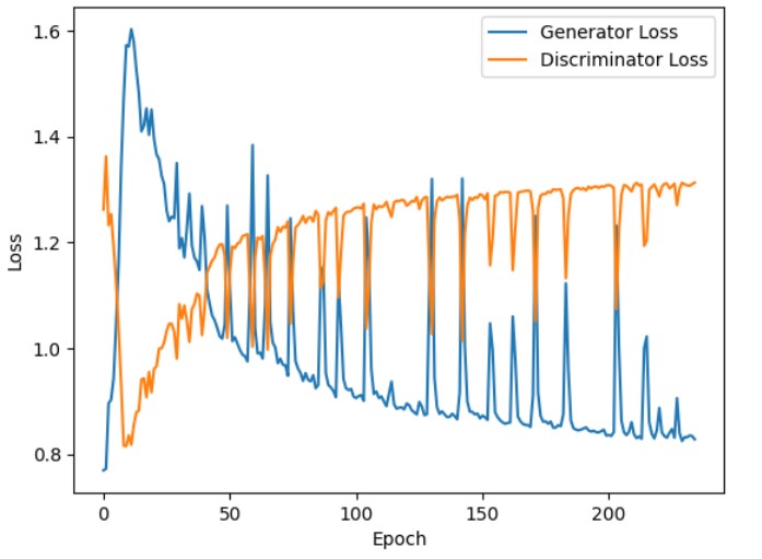
Figure 6: Generator and discriminator losses during training
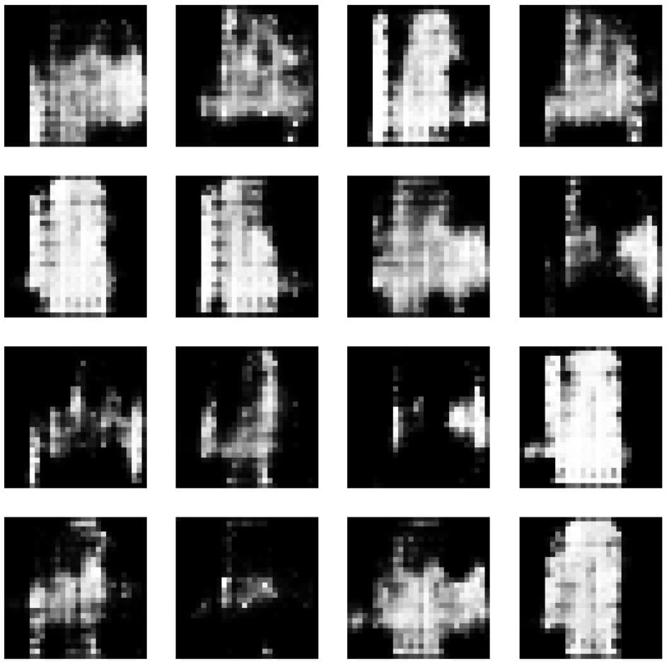
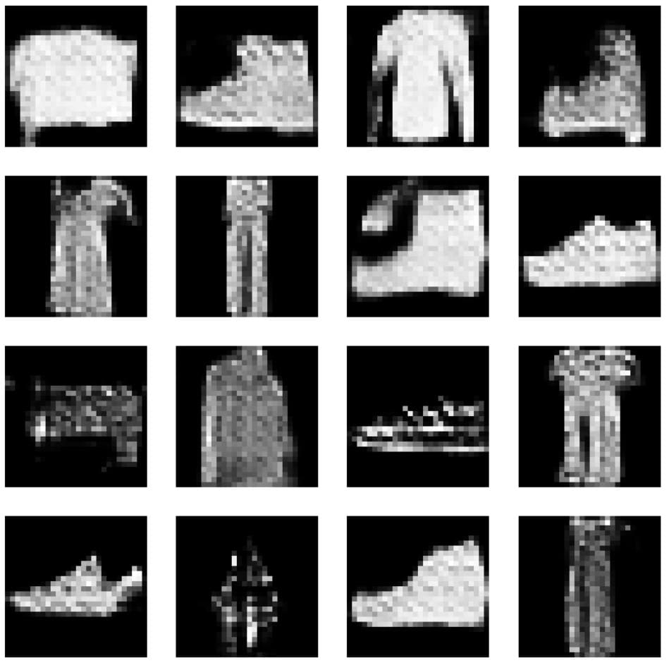
The figure below shows the images generated during training at the 10th, 50th, 150th, and 300th epochs (Figure 7). We observe that the quality of the generated images is improving as the training progresses. The image generated after 300 epochs seems to be quite similar to the fashion MNIST dataset.
(a) Epoch=10
(b) Epoch=50
(c) Epoch=150
(d) Epoch=300
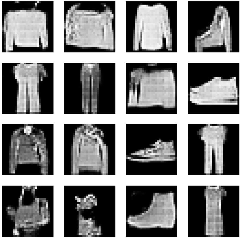
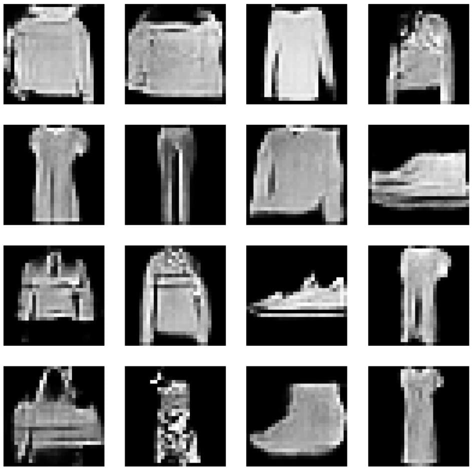
Figure 7: GAN-generated images at different epochs (10, 50, 150, and 300)
Conclusions
In this article, we learned the general architecture of GAN and the interplay between the different components of GAN. We also developed a GAN model using Tensorflow and Karas to generate synthetic fashion images that closely resemble real-world examples. Results demonstrate that the Gan model effectively captures intricate patterns and textures characteristic of fashion MNIST, such as clothing and accessories.
However, it is important to remember that GANs, like other machine learning models, also have their own challenges. While developing a GAN, we must be careful to properly tune model parameters and training techniques, which can be complex and time-consuming. However, with patience and persistence, the benefits of using GANs can be significant.
The potential applications of GANs are vast and diverse, although they come with many challenges. We can use GANs to generate realistic images, assist with data augmentation, and enhance privacy in data generation. GANs will continue to expand the horizons of what is possible in machine learning.