Overview
Have you ever wondered how artificial neural networks learn from data and perform complex tasks such as recognizing images, understanding natural languages, or driving cars?
If so, you might be interested in learning the feed forward neural network, one of the most popular and simplest types of neural networks.
A feed-forward neural network consists of one input layer, one or more hidden layers, and one output layer. This article will help you to understand the basics of feed forward neural networks, their structure and terminology, activation functions of feed forward neural networks, loss functions, and training techniques.
With the help of this article, you will be able to develop and train your first feed forward neural network model for classifying the fashion MNIST dataset. Once you finish the article, you will have an in-depth understanding of the feed forward neural networks. Let’s dive into the article and learn how to implement a feed forward network in Python using TensorFlow.
Understanding Feed forward Neural Network
A feedforward neural network is a type of artificial neural network consisting of one input layer, one or more hidden layers, and one output layer. In the feedforward networks, information flows forward from the input layer to the output layer through hidden layers.
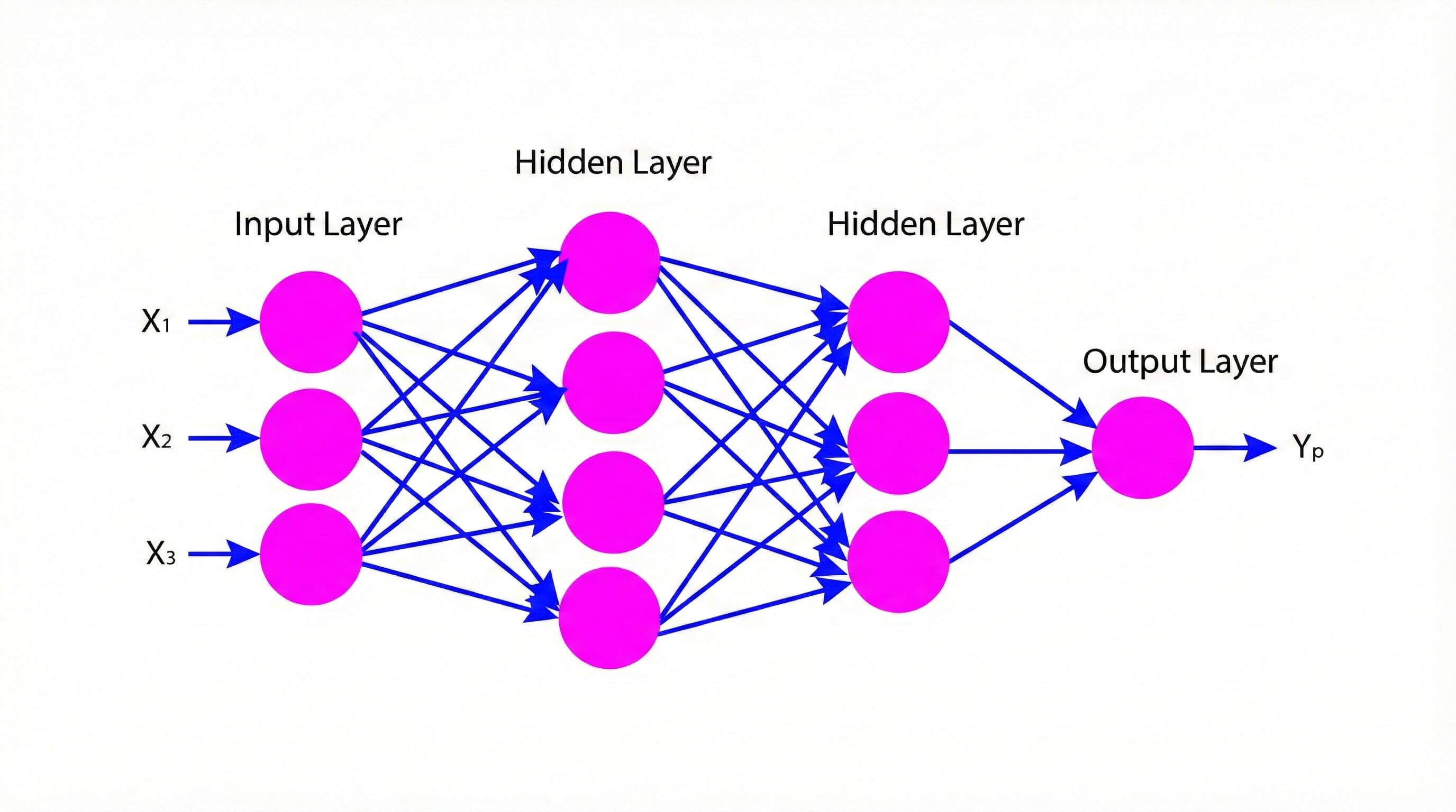
The figure below shows a pictorial representation of the feed forward neural network consisting of various layers: input layer, hidden layers, and output layer (Figure 1). Let us try to understand the various components of the feedforward network one by one:
Figure 1: Pictorial representation of feed forward neural networks
Input Layer
An input layer consists of several neurons or nodes that receive input features and pass them to the nearby hidden layer. The number of neurons in the input layer is determined by the number of input features.
Hidden Layers
The hidden layers in the feed forward neural networks are the intermediate layers between the input and output layers. They are used to perform transformations on the inputs with the help of non-linear functions to the weighted sum of the inputs. By doing so, the network learns complex patterns in the data and extracts useful features.
The output of each hidden layer is passed on to the next hidden layer or the output layer. In the above figure, there are two hidden layers. We can adjust the number of hidden layers and the number of neurons in each layer based on the complexity of the problem that needs to be solved.
Output Layer
The output layers consist of neurons or nodes that receive inputs from the last hidden layer and produce the final output. The number of neurons in the output layer equals the number of output features. For example, suppose you want to build a neural network model to identify the images into different categories, such as cats and dogs. In this case, the number of neurons in the output layer will equal the number of categories, which is two here.
Weights And Biases
The weights and biases are the learnable parameters in a feedforward neural network. These parameters are important for the network to learn and make accurate predictions.
Weights are numerical values that determine the strength of the connections between neurons from different layers.
Biases are constant values added to the weighted sum of the inputs in a neural network. They are a form of threshold or offset, and they allow neurons to activate even when the weighted sum of their inputs is not sufficient on its own.
Activation Functions
Activation functions are applied to the output of each neuron to help the network learn complex patterns (nonlinear relationships) in the data.
There are various types of activation functions such as sigmoid, tanh, ReLU (Rectified Linear Unit), Leaky ReLU, ELU (Exponential Linear Unit), and many more.
The performance of a neural network model highly depends on the choice of activation function. The RELU is one of the popular and widely adopted activation functions in deep learning.
We need to carefully consider the unique requirements of the network and the nature of the problem to be solved while selecting an activation function.
Loss Functions
The loss function is a mathematical function that helps us to measure how well a neural network model performs on a certain task. A neural network model improves its predictive performance by minimizing the value of the loss function.
We can compute the loss function by measuring the difference between the actual output and the predicted output of a neural network model. For regression problems, the commonly used loss function is the mean squared error (MSE) while for classification problems, we can use cross-entropy as the loss function.
Backpropagation Algorithm
The backpropagation algorithm is one of the commonly used methods to train feedforward neural networks. There are two steps in backpropagation: forward propagation and backward propagation.
In forward propagation, the network is fed input data, and the output is calculated. The backward propagation then checks the error between the predicted and actual output and propagates the error back through the network by updating the weights and biases. The algorithm uses gradient descent optimization to update the weights and biases.
Practical Implementation in Python with TensorFlow
Let us develop a feed-forward neural network model in Python to classify images of clothing items from the Fashion MNIST dataset. We will use TensorFlow and Keras, a high-level API for building and training models in TensorFlow. You can also find the sample code in the following link: FFNN.
Understanding The Dataset
The fashion MNIST dataset is a very popular and reliable dataset for training and evaluating the performance of various machine learning and deep learning models. In this dataset, there are 60,000 training examples and 10,000 testing examples.
Each example in the dataset is a grayscale image of 28 pixels in height and 28 pixels in width. Thus, the total pixels in a single image is 784.
Each pixel is associated with a single pixel value, an integer within the range [0, 255]. The pixel value represents the intensity of the pixel, with 0 being the minimum intensity (black) and 255 being the maximum intensity (white).
The images are labeled as 0-9, indicating their clothing categories, which are: T-shirt/top [0], Trousers [1], Pullover [2], Dress [3], Coat [4], Sandal [5], Shirt [6], Sneaker [7], Bag [8], and Ankle boot [9].
There are 785 columns in the dataset. The first column contains the labels of the clothing categories, and the rest of the columns have the pixel values of the associated image.
We can access a specific pixel in an image using the following formula:
Where x is an integer within the range [0, 783]; i and j are also integers within the range [0, 27]
Import Libraries
Let us import the necessary libraries.
import datetime
import numpy as np
import tensorflow as tf
from tensorflow.keras.datasets import fashion_mnist
Load Datasets
The code snippet below loads the Fashion MNIST dataset and splits the data into training and test sets.
(X_train, y_train), (X_test, y_test) = fashion_mnist.load_data()Data Processing
Normalize The Data
Here, we normalize the pixel values of the images from the range of 0-255 to 0-1. The normalization step is essential to maintain the pixels of all the images within a uniform range.
X_train = X_train / 255.0
X_test = X_test / 255.0
Reshape Data
The code snippet below reshapes the training and testing data from 2D arrays of 28×28 pixels to 1D arrays of 784 pixels. By doing so, we flattened the images to make them compatible with machine learning models, which expect 1D input vectors.
X_train = X_train.reshape(-1, 28*28)
X_test = X_test.reshape(-1, 28*28)
Build Feedforward Neural Network (FFNN) Model
Here, we will build a feed forward neural network using Keras.
model = tf.keras.models.Sequential()model.add(tf.keras.layers.Dense(units=256, activation='relu', input_shape=(784, )))model.add(tf.keras.layers.Dropout(0.25))model.add(tf.keras.layers.Dense(units=128, activation='relu'))model.add(tf.keras.layers.Dropout(0.25))model.add(tf.keras.layers.Dense(units=10, activation='softmax'))Compile Model
We will compile the model using adam optimizer.
model.compile(optimizer='adam', loss='sparse_categorical_crossentropy', metrics=['sparse_categorical_accuracy'])Train Model
Train The model for 20 epochs.
model.fit(X_train, y_train, epochs=20)The output window below shows the results of the last five epochs during training. We observe that the accuracy of the model after 20 epochs is 90.74%.
Output:
Epoch 15/20
1864/1875 [============================>.] - ETA: 0s - loss: 0.2622 - sparse_categorical_accuracy: 0.9018GPU utilization: 20 %
1875/1875 [==============================] - 5s 3ms/step - loss: 0.2623 - sparse_categorical_accuracy: 0.9018
Epoch 16/20
1868/1875 [============================>.] - ETA: 0s - loss: 0.2637 - sparse_categorical_accuracy: 0.9016GPU utilization: 19 %
1875/1875 [==============================] - 6s 3ms/step - loss: 0.2637 - sparse_categorical_accuracy: 0.9015
Epoch 17/20
1858/1875 [============================>.] - ETA: 0s - loss: 0.2601 - sparse_categorical_accuracy: 0.9021GPU utilization: 21 %
1875/1875 [==============================] - 5s 3ms/step - loss: 0.2599 - sparse_categorical_accuracy: 0.9022
Epoch 18/20
1873/1875 [============================>.] - ETA: 0s - loss: 0.2529 - sparse_categorical_accuracy: 0.9047GPU utilization: 16 %
1875/1875 [==============================] - 6s 3ms/step - loss: 0.2528 - sparse_categorical_accuracy: 0.9047
Epoch 19/20
1868/1875 [============================>.] - ETA: 0s - loss: 0.2521 - sparse_categorical_accuracy: 0.9039GPU utilization: 21 %
1875/1875 [==============================] - 5s 3ms/step - loss: 0.2518 - sparse_categorical_accuracy: 0.9039
Epoch 20/20
1866/1875 [============================>.] - ETA: 0s - loss: 0.2471 - sparse_categorical_accuracy: 0.9072GPU utilization: 14 %
1875/1875 [==============================] - 5s 3ms/step - loss: 0.2467 - sparse_categorical_accuracy: 0.9074
Evaluate Model Performance
Let us evaluate the model performance on the test dataset.
y_test = np.array(y_test, dtype=int)
test_loss, test_accuracy = model.evaluate(X_test, y_test)313/313 [==============================] - 1s 2ms/step - loss: 0.3170 - sparse_categorical_accuracy: 0.8927We observe that the model’s accuracy for the test dataset is 89.27%, which is quite good.
Conclusions
In this article, we explored the various fundamental details of feed forward neural networks (FFNNs) and their implementation using Keras. We covered various topics, such as the architecture of FNNs, activation functions, loss functions, and optimization techniques. We build a feed forward neural network using KERAS to classify clothing items from the Fashion MNIST dataset.
We hope you gained valuable knowledge about the feed forward neural network (FFNN) by exploring this article. Learning feed-forward neural networks will provide you with a strong foundation for more complex neural network architectures.
We also suggest experimenting with various architectures, hyperparameters, and datasets to enhance your comprehension and improve model performance. Happy coding, and may your neural networks thrive!
Frequently Asked Questions
What is a feed forward neural network?
A feedforward network (FFNN) is an artificial neural network consisting of an input layer, one or more hidden layers, and an output layer. In a feedforward network, the information moves only in the forward direction (from input to output) without forming loops. Backpropagation algorithms are typically used to train the feed-forward network. This straightforward architecture is widely used for various tasks such as classification and regression.
How does a feedforward neural network work?
In a feedforward neural network, connections between nodes do not form a cycle. Information moves only in the forward direction from the input nodes through the hidden nodes (if any) to the output nodes. In each node, a weighted sum of the inputs is passed through an activation function, and the output is sent to the next layer. This process is repeated until the output layer is reached, providing the final prediction of the network.
Is CNN a feed forward neural network?
A Convolutional Neural Network (CNN) is a type of feedforward neural network used to process grid-like data such as images. A CNN consists of convolutional layers to identify patterns in the images and pooling layers to reduce the dimensionality of the data. The data flows only in the forward direction, from the input to the output layer, through hidden layers.
References
Feed Forward neural Network Basics
Introduction To Feed Forward Neural Network