Overview
Don’t you think it is incredible that self-driving cars can detect pedestrians, traffic signs, obstacles, and other objects on the road? How do they observe the surroundings and make decisions? The secret behind such an amazing feat lies in the powerful technique known as convolutional neural networks (CNNs), which serves as the backbone of many such computer vision applications.
Convolutional neural networks (CNNs) are not limited to computer vision but also various other domains such as natural language processing, speech recognition, audio analysis, medical image analysis, and many more. CNNs can handle complex and high-dimensional data better than traditional machine learning models. Moreover, CNNs are robust to noise and variations and have better generalization ability on new and unseen data.
This article will explore the background of convolutional neural networks, their various components, hyperparameters, and some popular architectures. So, let’s dive in and learn everything about CNNs in this amazing article.
Background Of Convolutional neural networks
It all started in the 1980s when Kunihiko Fukushima and his research group proposed the Neocognitron, which is a hierarchical network of simple and complex cells to recognize handwritten characters. However, in those days, it did not receive enough attention due to their computational burden and limited availability of data. The applications of neural networks were limited to recognizing handwritten characters such as postal codes and bank checks.
However, a breakthrough happened in 2012 when Alex Krizhevsky and his colleagues developed a convolutional neural network model called AlexNet and won ImageNet (which was a large-scale image recognition competition). Their model achieved a remarkable performance by outperforming the previous state-of-the-art by a large margin.
With the breakthrough of AlexNet, great interest was renewed in convolutional neural networks and deep learning. Researchers around the world understood the significance and potential of convolutional neural networks to handle complex and diverse tasks, such as object detection, face recognition, natural language processing, and many others.
Understanding Convolutional Neural Networks
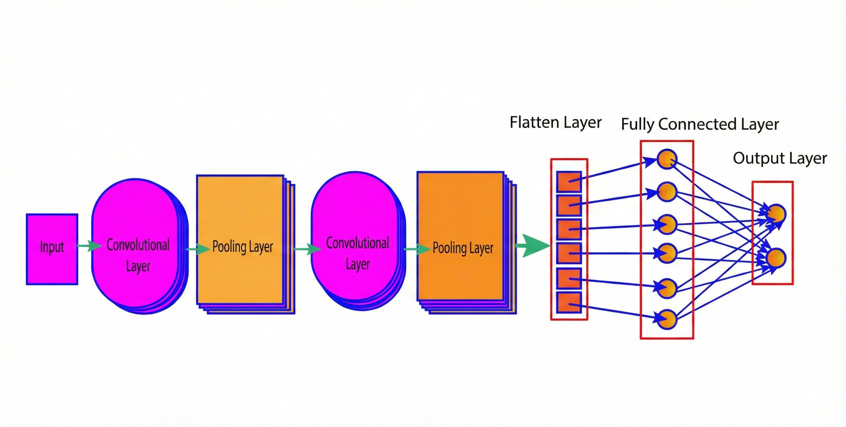
Convolutional Neural Networks (CNN) is a type of deep learning algorithm for analyzing images. It has multiple layers (shown in the figure below) each serving a specific purpose in the feature extraction and pattern recognition process. The section below discusses various components of CNN in detail.
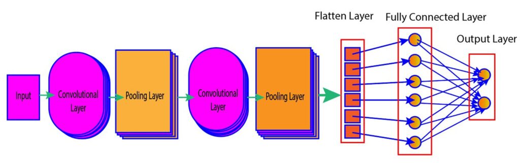
Figure 1: Various layers of convolutional neural networks
Convolutional Layer
In the convolutional layer, filters are applied to the input image to extract specific features such as edges, shapes, and patterns. The extracted features are also known as feature maps, which indicate the locations and strengths of the features in the image. The process of extracting important features from images is also known as the convolution operation.
In the convolution operation, a filter (which is also known as a kernel and is typically a 3×3 or 5×5 matrix) slides over the input matrix repetitively, producing the dot product (element-wise multiplication and summation) of the input pixels and the filter values. The dot product is stored in an output matrix, also known as a feature map.
In the next step, the filter is shifted by a certain number of pixels, called the stride, and the above process is repeated until the filter has swept across the entire image.
Let us try to visualize the convolution operation with the help of the figure below (Figure 2). In the figure, we have a filter of size 3×3 matrix that slides over the input image, which is a 5×5 matrix. In the first step, the filter starts from the top-left corner of the input image and multiplies each element of the filter with the corresponding element of the input image. Then, it adds all the products and stores the sum in the feature map. The value of the feature map is found to be 22 in this case.
In the second step, the filter is moved one pixel to the right, and after the convolution operation, the value of the feature is found to be 15.
This process needs to be repeated until the filter covers the entire input image, resulting in a 3×3 feature map. This is how the convolution operation between the input images and filters takes place.
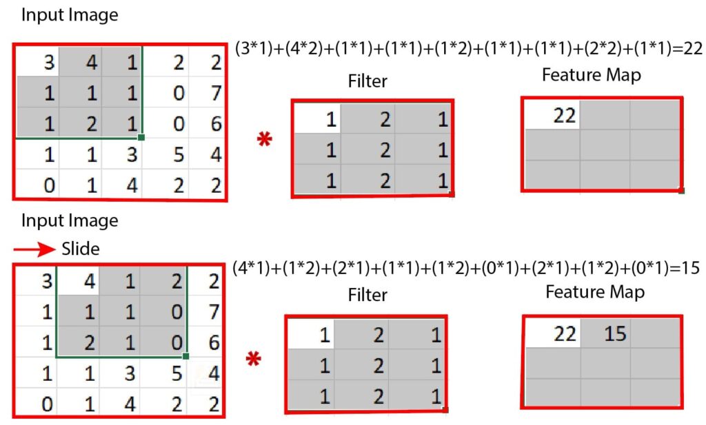
Figure 2: Illustration of the convolution operation
Activation Layer
In convolutional neural networks, an activation layer such as ReLU (Rectified Linear Unit) is generally applied after each convolutional layer. It adds non-linearity to the model by transforming the output of the convolutional layer. By doing so, the network learns complex patterns between the features in the image and generalizes better.
The activation layer also helps to alleviate the vanishing gradient problem, which may impede the training of deep neural networks.
Pooling layer
The pooling layer is used to reduce the spatial dimension of the feature map by applying the pooling operation. Similar to the convolution layers, the pooling layers also use filters to scan the input. However, the pooling layers don’t have learnable parameters, unlike convolution layers.
Instead, they compute the maximum or the average value of the pixels within the filter and populate an output array using those values. There are two common types of pooling operations: max pooling and average pooling.
Max pooling
The max pooling selects several small subregions in the feature map, finds the maximum in those regions, and uses it to create a pooled (downsampled) feature map. Figure 3 illustrates the max pooling operation. There are several advantages of max pooling:
-
Max pooling reduces the number of parameters and computations in the model, making it computationally efficient.
-
Max pooling improves the generalization ability by making the model less sensitive to the location and orientation of features in the input.
-
Max pooling helps to avoid overfitting by suppressing noise and irrelevant details in the input, which leads to better detection of dominant features.
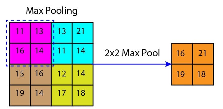
Figure 3: Max pooling
Average pooling
The average pooling selects several small subregions in the feature map, computes the average of the pixels in those regions, and uses it to create a pooled (downsampled) feature map. Figure 4 illustrates the average pooling operation. There are several advantages of average pooling:
-
Average pooling improves the robustness of the model by reducing the effect of background noises and outliers in the feature map.
-
Average pooling improves the computational performance by reducing the number of parameters in the model.
-
Average pooling smooths the feature map and reduces the variance, which helps to extract more global features from the input.
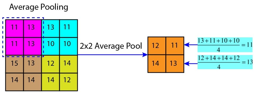
Figure 4: Average pooling
Fully Connected Layer
In the fully connected layer, each neuron in a layer is connected to all the neurons in the previous layer. This layer takes the flattened output of the last convolutional or pooling layer as input and performs the final classification or regression task.
The fully connected layer can have multiple hidden layers, each with a different number of neurons and activation functions. The activation function in the fully connected layer helps to introduce non-linearity and map the output in the desired range. Some of the common activation functions are tanh, ReLU, softmax, and sigmoid.
Hyperparameters
Hyperparameters are the parameters that determine the network structures and training processes of convolutional neural networks. These parameters must be set before training and cannot be calculated from the data. Various hyperparameters of CNN are:
Number Of Hidden Layers And Units
The number of hidden layers determines the depth of the network, and the number of units in each layer determines the width of the network. A deeper network is capable of learning more complex features. However, it is prone to overfitting. A wider network is computationally expensive, although it can learn more diverse features.
The optimal number of hidden layers and units depends on the complexity of the problem and the size of the dataset. We can start with a small number of hidden layers and units and increase them gradually while checking whether they improve the performance of the model.
Number Of Filters In Each layer
A filter is a small matrix of 3×3 or 5×5 matrix which slides over the input pixels to extract important features. The number of feature maps in the output layers depends on the number of filters. A larger number of filters can capture diverse features but at the expense of computational performance.
The optimal number of filters depends on the size of the dataset and the complexity of the problem. We can start with a small number of filters and increase them gradually until the performance plateaus or starts to degrade.
Learning Rate
The learning rate controls how much to update the weight in the optimization algorithm. It determines the step size of the gradient descent algorithm. Choosing a high learning rate can cause the algorithm to overshoot the minimum, while a low learning rate can cause the algorithm to converge slowly.
The optimal learning rate depends on the problem and the network architecture. In practice, we can start with a small learning rate and increase it gradually until the performance stabilizes or starts to decline.
Regularization
The regularization technique helps to avoid overfitting in the network or reduce variance in the network by penalizing it for complexity. In the regularization technique, a penalty term is added to the loss function, which allows to discourage large weights. The two most common regularization techniques are the L1 regularization and L2 regularization.
In the L1 regularization, the absolute value of the weights is added to the loss function. On the other hand, the L2 regularization adds the square of the weights to the loss function. The L2 regularization is more common in convolutional neural networks.
The optimal strength of the regularization depends on the problem and the architecture of the network. We can start with a small regularization strength and increase it gradually until the performance starts decreasing or stabilizes.
Dropout
In the dropout, some units of the network are dropped randomly, forcing the network to learn more robust features and avoid overfitting. A common practice is to start with a small dropout and increase it gradually until the performance stops improving or stabilizes.
Padding
Padding is used to preserve the spatial information of the input image at the borders that might be lost during convolution operation.
In the padding, zeros are added around the edges of the input image, which helps feature maps to maintain their spatial size without losing information. For example, the figure below illustrates padding on an input image of size 3×3 (Figure 5). The resulting image after padding is an image of size 5×5.
There are mainly two types of padding in convolution neural networks:
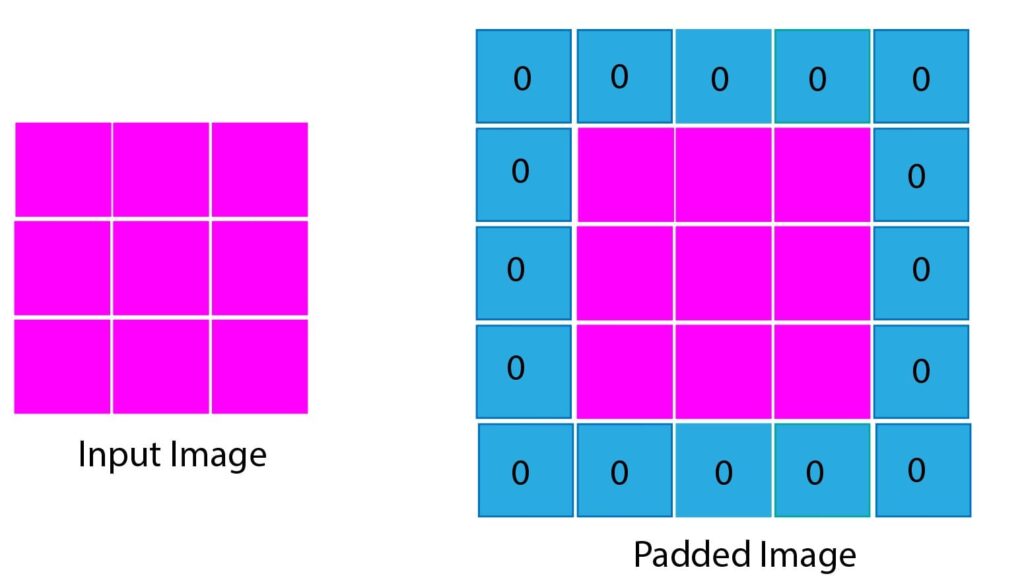
Figure 5: Padding example in convolutional neural networks
Valid Padding
Valid padding does not add any extra pixels to the input image before applying convolution. As a result, the output feature map is smaller than the input data.
Valid padding is useful when we want to reduce the dimensionality of the feature map. However, we might lose some information about images at the border due to the filter size in the valid padding.
Same Padding
In the same padding, we want to preserve the spatial dimension of the input image and don’t want to lose information at the edge of the image. The output feature map in the same padding has the same spatial dimensions as the input image.
In the same padding, we add rows and columns of pixels around the edge of the input image. This helps to retain important features and avoid shrinking the image too much.
Popular Architectures of Convolutional Neural Network
Over the years, many variants of convolutional neural networks have been developed, each with different design choices and trade-offs. Here, we will discuss some of the most influential and popular architectures of Convolutional neural networks.
LeNet-5
It is one of the first architectures of convolutional neural networks , which was introduced in 1998. This architecture is widely used for handwritten digit recognition. It has two convolutional layers, three fully connected layers, and about 60,000 parameters.
We can also process higher-resolution images in LeNet-5 by adding more convolutional layers.
AlexNet
This architecture led a breakthrough in the field of deep learning by winning the famous ImageNet competition in 2012. The architecture was designed by Alex Krizhevsky and his research group at the University of Toronto.
In the AlexNet model, there are five convolutional layers, three fully connected layers, and about 60 million parameters. The activation function used in AlexNet is the rectified linear units, while dropout is used as a regularization technique. AlexNet also uses data augmentation to increase the diversity of the training data.
VGG
VGG is a popular deep convolutional neural network architecture developed by the Visual Geometry Group at the University of Oxford in 2014. Two main variants of VGG are VGG-16 and VGG-19, which have 16 and 19 layers, respectively.
The VGG architecture typically consists of multiple convolution layers and fully connected layers. For example, the VGG-16 model has 13 convolutional layers, three fully connected layers, and 38 million parameters.
GoogLeNet
GoogLeNet is a 22-layered deep convolutional neural network developed by researchers at Google in 2014. It won the ImageNet Challenge 2014. GoogLeNet uses techniques such as 1×1 convolutions in the middle of the architecture and inception modules. This allows the GoogLeNet to select multiple convolutional filter sizes in each block.
In the GoogLeNet, there are a total of 9 inception blocks arranged into three groups with max-pooling in between and global average pooling in its head to generate its estimate.
The global average pooling layer of the GoogLeNet network also helps to combat the gradient vanishing problem.
EfficientNet
EfficientNet was developed by Google AI researchers in 2019. The architecture is based on “compound scaling” that addresses the trade-off between computational efficiency and model performance in deep learning.
EfficientNet combines depth-wise separable convolutions and inverted residual blocks called Mobile Inverted Bottleneck layers. The performance of the architecture can be improved using the global average pooling layer and the Squeeze-and-Excitation optimization method.
Frequently Asked Questions
What is a Convolutional Neural Network (CNN)?
A Convolutional Neural Network (CNN) is a type of artificial neural network that can be used to analyze visual data, such as images and videos. We can use CNN for various tasks such as image classification, object detection, natural language processing, time series analysis, medical imaging, and segmentation. The convolutional layers help it learn hierarchical features from input images in CNN.
How do CNNs handle color images?
CNN treats color images as three separate channels corresponding to the Red, Green, and Blue (RGB) components. Each channel is processed independently by applying convolutional filters to learn features and patterns specific to that color channel. CNN then combines learned features from all three channels, which effectively helps recognize the objects and patterns in the color images.
What is the main application of CNN?
Convolutional neural networks (CNNs) are used for various computer vision tasks such as image recognition, object detection, facial recognition, medical image analysis, self-driving cars, video analysis, and more. They also play an important role in medical image analysis by helping in the diagnosis of diseases through the interpretation of X-rays, MRIs, and other medical scans. CNN also helps self-driving cars understand and navigate their environment by processing visual data.
Conclusions
In this article, we discussed various components of convolutional neural networks (CNNs), such as convolutional, activation, pooling, and fully connected layers.
We also discussed various hyperparameters that may help to avoid overfitting, improve generalization ability to new data, and improve computational performances.
This article also provided a brief overview of various popular architectures of CNNs, such as LeNet-5, AlexNet, VGG, GoogLeNet, and EfficientNet, each with different design choices and trade-offs.
We hope you liked this article. If you want to learn how to implement convolutional neural networks in TensorFlow to classify images, then you might check this tutorial.