Overview
Do you want to learn how to develop a powerful convolutional neural network (CNN) in TensorFlow that can recognize images from 10 different categories? If this is the case, then you are in the right place. In this article, I will help you to create and train a CNN in TensorFlow to classify the CIFAR-10 dataset into different categories.
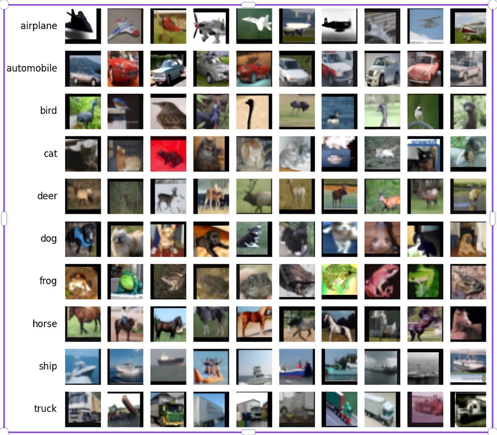
The CIFAR-10 is a popular dataset in deep learning, consisting of 60,000 colorful images. The images belong to ten categories: airplane, automobile, bird, cat, deer, dog, frog, horse, ship, and truck. The aim is to develop a CNN in TensorFlow to classify images into different categories.
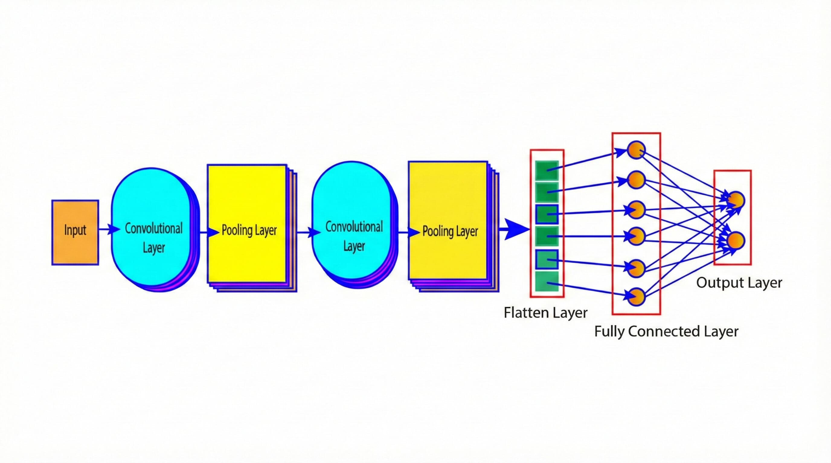
For those who are not aware of what CNNs are, they are a type of deep learning algorithm involving multiple layers of filters to extract important features from the input images. They are one of the most effective deep-learning models for recognizing patterns and shapes in images, and they have achieved state-of-the-art results on many image recognition tasks. If you want to know more about CNN, you can check our previous tutorial on CNN, which discusses its associated theories.
In this article, you will learn how to:
-
Load and preprocess the CIFAR-10 dataset using TensorFlow
-
Build a CNN in TensorFlow from scratch by using the KERAS API
-
Train and evaluate the performance of the model on the training and test datasets
-
Explore some ways to improve the model’s performance and accuracy
By developing a CNN in TensorFlow, one can also benefit from the rich documentation and community support that TensorFlow provides. Once you finish the article, you will have a solid understanding of the practical implementation of CNN in TensorFlow. So, let’s develop your first CNN model in TensorFlow for image classification.
What Is TensorFlow?
TensorFlow is an open-source software library developed by researchers at Google for running machine learning and artificial intelligence applications.
We can develop a CNN model in TensorFlow for various tasks such as image classification, detection, and segmentation. There are various approaches to developing a CNN in TensorFlow, such as the Keras Sequential API, the Functional API, or the low-level TensorFlow Core API.
TensorFlow has high-level APIs, such as Keras and tf.keras.layers, and using them, we can quickly build and train CNNs with just a few lines of code. It also supports low-level APIs that offer a lot of flexibility and customization of CNNs, such as defining loss functions, optimizers, and custom layers.
TensorFlow also offers many pre-trained CNN models, such as VGG-16, ResNet50, Inceptionv3, and EfficientNet1. These pre-trained models can be easily fine-tuned and used as feature extractors for new tasks.
Understanding The CIFAR-10 Dataset
CIFAR-10 is a dataset of 60,000 color images collected in 2009 by Alex Krizhevsky, Vinod Nair, and Geoffrey Hinton. The dataset is popular for evaluating and comparing different image classification models, such as convolutional neural networks (CNNs), residual networks, dense networks, and capsule networks. Using the CIFAR-10 dataset, we can develop our own CNN in TensorFlow for image classification.
The dataset is split into 50,000 color images of 32×32 pixels for training and 10,000 color images of 32×32 pixels for testing.
Each image of the dataset is an array of 3072 elements, representing 32×32 pixels of the red, green, and blue channels. The dataset is divided into tenclasses: airplane [0], automobile [1], bird [2], cat [3], deer [4], dog [5], frog [6], horse [7], ship [8], and truck [9].
The dataset also permits various data augmentation techniques such as cropping, flipping, rotating, and adding noise. These augmentation techniques can be used to improve the generalization and robustness of the models. The figure below illustrates the various classes of images in the CIFAR-10 dataset.

Figure 1: Sample images from the CIFAR-10 dataset
Practical Implementation Of CNN In TensorFlow
Here, we will develop a CNN in TensorFlow for recognizing images in the CIFAR-10 Dataset. You can find the source code here: CNN in Tensorflow.
Import Libraries
import matplotlib.pyplot as plt
import tensorflow as tf
from tensorflow.keras.datasets import cifar10
Data Processing
Data processing is an essential step to develop a CNN in TensorFlow. It involves the following steps.
Load Data
(X_train, y_train), (X_test, y_test) = cifar10.load_data()Normalize The Data
The normalization reduces the variance and skewness of the data, which helps the model to learn fast, improves generalization ability, and enhances model performance on unseen data. Here, we will divide the pixels of the images by 255 to scale them within the range [0,1].
X_train = X_train / 255.0
X_test = X_test / 255.0print(X_train.shape)Output:
(50000, 32, 32, 3)print(X_test.shape)Output:
(10000, 32, 32, 3)Build CNN Model
Here’s a step-by-step guide on how to create a CNN in TensorFlow.
Define Model
model = tf.keras.models.Sequential()CNN Layer 1
Add a 2D convolution layer with 32 filters, 3×3 kernel size, same padding, and ReLU activation function. The input shape is 32x32x3.
model.add(tf.keras.layers.Conv2D(filters=32, kernel_size=3, padding="same", activation="relu", input_shape=[32, 32, 3]))CNN Layer 2
Add a second 2D convolution layer with 32 filters, 3×3 kernel size, same padding, and ReLU activation function.
model.add(tf.keras.layers.Conv2D(filters=32, kernel_size=3, padding="same", activation="relu"))Max Pooling Layer 1
Add a max pooling layer to downsample the input along its spatial dimensions by taking the maximum value over a pool size 2×2, with a stride of 2 and no padding.
model.add(tf.keras.layers.MaxPool2D(pool_size=2, strides=2, padding='valid'))CNN Layer 3
Add a 2D convolution layer with 64 filters, 3×3 kernel size, same padding, and ReLU activation function.
model.add(tf.keras.layers.Conv2D(filters=64, kernel_size=3, padding="same", activation="relu"))CNN Layer 4
Add a 2D convolution layer with 64 filters, 3×3 kernel size, same padding, and ReLU activation function.
model.add(tf.keras.layers.Conv2D(filters=64, kernel_size=3, padding="same", activation="relu"))Max Pooling Layer 2
Add a max pooling layer to downsample the input along its spatial dimensions by taking the maximum value over a pool size 2×2, with a stride of 2 and no padding.
model.add(tf.keras.layers.MaxPool2D(pool_size=2, strides=2, padding='valid'))Flatten Layer
Flattening helps to convert the input into a one-dimensional array. The one-dimensional array can now be fed directly to a dense layer.
model.add(tf.keras.layers.Flatten())Dense layer 1
Add a dense layer with 128 output neurons and the ReLU activation function.
model.add(tf.keras.layers.Dense(units=128, activation='relu'))Dense layer 2
Add a dense layer with ten output neurons and the “softmax” activation function. The**“softmax”** activation function is used here for multi-class classification, which normalizes the output into a probability distribution over the different classes.
model.add(tf.keras.layers.Dense(units=10, activation='softmax'))Model Summary
We can visualize the architectures and various parameters of the CNN in Tensorflow
model.summary()Output:
_________________________________________________________________
Layer (type) Output Shape Param #
=================================================================
conv2d (Conv2D) (None, 32, 32, 32) 896
max_pooling2d (MaxPooling2 (None, 16, 16, 32) 0
D)
conv2d_1 (Conv2D) (None, 16, 16, 64) 18496
conv2d_2 (Conv2D) (None, 16, 16, 64) 36928
max_pooling2d_1 (MaxPoolin (None, 8, 8, 64) 0
g2D)
flatten (Flatten) (None, 4096) 0
dense (Dense) (None, 128) 524416
dense_1 (Dense) (None, 10) 1290
=================================================================
Total params: 582026 (2.22 MB)
Trainable params: 582026 (2.22 MB)
Non-trainable params: 0 (0.00 Byte)
_________________________________________________________________Compile The Model
Here, we compile the model using sparse categorical cross-entropy as the loss function, Adam as the optimization algorithm, and sparse categorical accuracy as the evaluation metric.
model.compile(loss="sparse_categorical_crossentropy", optimizer="Adam", metrics=["sparse_categorical_accuracy"])Train The Model
Let us train the CNN in TensorFlow with 15 epochs.
model.fit(X_train, y_train, epochs=15)The output below shows that the model has a loss of 0.1226 and a sparse categorical accuracy of 0.9550. This means the model can predict the class of the training samples with 95.5% accuracy.
Output:
Epoch 1/15
1563/1563 [==============================] - 12s 5ms/step - loss: 1.3854 - sparse_categorical_accuracy: 0.5037
Epoch 2/15
1563/1563 [==============================] - 6s 4ms/step - loss: 0.9805 - sparse_categorical_accuracy: 0.6563
Epoch 3/15
1563/1563 [==============================] - 7s 5ms/step - loss: 0.8179 - sparse_categorical_accuracy: 0.7146
Epoch 4/15
1563/1563 [==============================] - 6s 4ms/step - loss: 0.6994 - sparse_categorical_accuracy: 0.7566
Epoch 5/15
1563/1563 [==============================] - 7s 5ms/step - loss: 0.5975 - sparse_categorical_accuracy: 0.7918
Epoch 6/15
1563/1563 [==============================] - 6s 4ms/step - loss: 0.5046 - sparse_categorical_accuracy: 0.8233
Epoch 7/15
1563/1563 [==============================] - 7s 5ms/step - loss: 0.4152 - sparse_categorical_accuracy: 0.8550
Epoch 8/15
1563/1563 [==============================] - 6s 4ms/step - loss: 0.3460 - sparse_categorical_accuracy: 0.8781
Epoch 9/15
1563/1563 [==============================] - 7s 5ms/step - loss: 0.2816 - sparse_categorical_accuracy: 0.9005
Epoch 10/15
1563/1563 [==============================] - 7s 4ms/step - loss: 0.2281 - sparse_categorical_accuracy: 0.9193
Epoch 11/15
1563/1563 [==============================] - 7s 4ms/step - loss: 0.1887 - sparse_categorical_accuracy: 0.9330
Epoch 12/15
1563/1563 [==============================] - 7s 4ms/step - loss: 0.1636 - sparse_categorical_accuracy: 0.9420
Epoch 13/15
1563/1563 [==============================] - 7s 4ms/step - loss: 0.1361 - sparse_categorical_accuracy: 0.9524
Epoch 14/15
1563/1563 [==============================] - 8s 5ms/step - loss: 0.1249 - sparse_categorical_accuracy: 0.9567
Epoch 15/15
1563/1563 [==============================] - 10s 7ms/step - loss: 0.1226 - sparse_categorical_accuracy: 0.9550
Evaluate The Model Performance And Predict
Let us evaluate the model performances on the test dataset.
test_loss, test_accuracy = model.evaluate(X_test, y_test)The output below shows the performance of the model on the test dataset. We observe that the model has achieved a loss of 1.7272 and a sparse categorical accuracy of 0.7128. In other words, the model can predict the categories of the test samples with 71.28% accuracy.
Output:
313/313 [==============================] - 1s 4ms/step - loss: 1.7272 - sparse_categorical_accuracy: 0.7128
Conclusions
In this article, we developed a CNN in TensorFlow to classify the images of the CIFAR-10 dataset into ten categories. We achieved an accuracy of about 70% on the test dataset, which is quite good for a simple CNN model.
We can further improve the performance of the model by adjusting various hyperparameters, such as increasing the number of layers or epochs and changing the learning rate.
We can also experiment with the dropout rates and batch normalization, which can help to strike a balance between overfitting and underfitting, improving the performance of the model.
Overall, the CNN in TensorFlow is a powerful and flexible tool for image recognition since it can learn complex features from data and adapt to different tasks and domains. We demonstrated how to build, train, and evaluate a CNN in TensorFlow by using the CIFAR-10 dataset. We hope this article inspires you to explore more applications of CNNs in TensorFlow and beyond.
Frequently Asked Questions
How many layers are in CNN?
Convolutional Neural Networks (CNNs) usually have multiple layers, such as convolutional, pooling, activation, and fully connected layers. A simple CNN model with basic architectures may have only a few layers, while a complex CNN model like VGG or ResNet can have dozens or even hundreds of layers.
Does CNN have fully connected layers?
Convolutional Neural Networks (CNNs) generally consist of convolutional layers, pooling layers, and fully connected layers (dense layers). The fully connected network is generally located at the end of the network. They help to gather learned features from previous layers and produce final predictions or classifications.
What is CNN in TensorFlow?
CNN in TensorFlow is a deep learning model that is mainly used for various image-related tasks such as object detection and classification. In a CNN model, convolutional layers are used to detect patterns, pooling layers for downsampling, and fully connected layers for high-level reasoning. With the help of TensorFlow API, we can build CNNs easily and efficiently.

