Unlock Computer Vision with AlexNet: Step-by-Step Tutorial

Overview

Are you curious about implementing one of the most impactful and pioneering deep learning models in computer vision? Look no further! In this article, we will guide you on how to build the AlexNet model, a convolutional neural network that won the 2012 ImageNet challenge and transformed the world of deep learning. We will use Keras, a high-level deep-learning API, to create and train the AlexNet model in Python.

The AlexNet model has five convolutional layers, three dense layers, and other features such as max pooling, dropout, and batch normalization.

The original AlexNet model used two parallel GPUs to train the network faster and overcome memory limitations. However, we will stick to a single GPU to keep the model simple. We will apply the model to classify cat and dog images.

In this article, you will learn the following:

A brief overview of the AlexNet network
How to preprocess the dataset involving cat and dog images
How to develop and compile the AlexNet model using Keras
How to train and evaluate the AlexNet model
How to visualize and interpret the results of the AlexNet model

The Birth Of AlexNet

Do you know that the year 2012 is considered a significant turning point in the field of artificial intelligence? This year, Alex Krizhevsky and his research group proposed AlexNet, a milestone in computer vision, particularly in image classification.

Before the invention of AlexNet, traditional machine-learning algorithms such as support vector machines and random forest algorithms were popular for image classification tasks. However, classifying images with the help of traditional machine-learning algorithms was a formidable challenge as they often found it difficult to extract important features from raw pixel data for datasets like ImageNet, which included millions of images across thousands of categories.

With the limitations of traditional machine-learning algorithms in mind, Krizhevsky and his team developed a new neural network architecture that broke records in the ImageNet challenge. AlexNet won the ImageNet Large Scale Visual Recognition Challenge (ILSVRC) in 2012 by a massive margin while achieving the top-5 error rate of 15.3%.

Understanding Alexnet Architecture

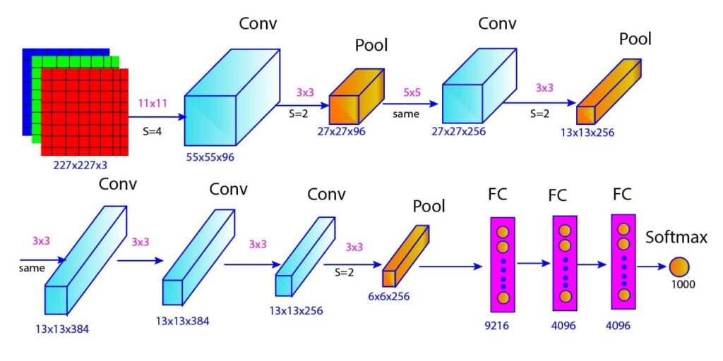
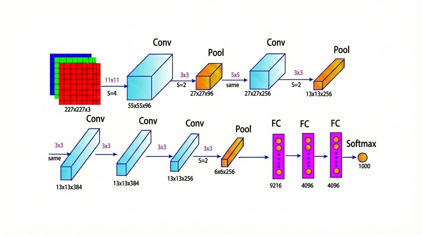
The AlexNet is a deep architecture consisting of five convolutional layers, three fully connected layers and one SoftMax output layer. The size of the input is 227x227x3, representing an RGB image. The output of the AlexNet model is a SoftMax layer that produces a probability distribution over 1000 categories, indicating the likelihood of the input image belonging to each category.

We can visualize the different layers and connections in AlexNet in the figure below. In the table below, we further provided the key details of each layer in AlexNet, including the type of layer, output size, kernel size, stride, and activation function used.

In the table below, we further provided the key details of each layer in AlexNet, including the type of layer, output size, kernel size, stride, and activation function used. In this blog post, we won’t discuss each layer one by one. Interested readers can follow our previous blog post for more detailed discussions on Alexnet architecture and its important features. Instead of going deep into the AlexNet architecture, we will focus on the implementation details of the AlexNet model to classify the cat and dog images using TensorFlow and Keras.

Layer	Type	Filter Size	Number of Filters	Stride	Padding	Output Size (WxHxD)	Activation
Input	-	-	-	-	-	227x227x3	-
Conv1	Convolutional	11x11	96	4	Valid	55x55x96	ReLU
Pool1	Max Pooling	3x3	-	2	0	27x27x96	-
Norm1	Local Response	-	-	-	-	27x27x96	-
Normalization
Conv2	Convolutional	5x5	256	1	2	27x27x256	ReLU
Pool2	Max Pooling	3x3	-	2	0	13x13x256	-
Norm2	Local Response	-	-	-	-	13x13x256	-
Normalization
Conv3	Convolutional	3x3	384	1	1	13x13x384	ReLU
Conv4	Convolutional	3x3	384	1	1	13x13x384	ReLU
Conv5	Convolutional	3x3	256	1	1	13x13x256	ReLU
Pool5	Max Pooling	3x3	-	2	0	6x6x256	-
FC6	Fully Connected	-	4096	-	-	4096	ReLU
Dropout	Dropout	-	-	-	-	4096	-
FC7	Fully Connected	-	4096	-	-	4096	ReLU
Dropout	Dropout	-	-	-	-	4096	-
FC8	Fully Connected	-	1000	-	-	1000	Softmax

Practical Implementation

Here, we will develop a model based on AlexNet architecture to classify a dataset containing images of dogs and cats. You can also download the dataset from this link. You can also check the whole code here.

Import Dependencies

Import the necessary modules for data preprocessing, model building, and image processing

				
					from sklearn.model_selection import train_test_split
import os
import tensorflow as tf
import pandas as pd
from keras.layers import BatchNormalization
from keras.models import Sequential
from keras.layers import Conv2D, MaxPooling2D, Flatten, Dense, Activation
from keras.layers import Dropout
from keras.preprocessing.image import ImageDataGenerator

Load Dataset

Here, we set the path to access the training and test dataset.

				
					train_path = os.getcwd() + '/' + 'train/'
test_path = os.getcwd() + '/' + 'test/'

				
					# Check Some Sample Image names In the Directory
image_names= os.listdir(train_path)
print(image_names[2],image_names[4000], image_names[13000],image_names[16000] )

				
					Output:
cat.9194.jpg cat.5634.jpg dog.8641.jpg dog.5985.jpg

Data Preprocessing

The code below will iterate through the list of images in the directory and extract their labels (either cat or dog).

				
					# Iterate Through A List Of Images and Extract Their Lables
label_list=[]
for image in image_names:
  label=image.split('.')[0]
  if (label=='cat'):
    label_list.append('cat')
  else:
    label_list.append('dog')

Save the image names and respective labels in a Pandas data frame.

				
					# Save Images and The respective labels In a Dataframe
df=pd.DataFrame({'imageName':image_names, 'label':label_list})
print(df)

Split the data into two parts: 75% of the data in the training set and 25% of the data in the validation set

				
					# Split The Dataset Into Training and Validation Data 
train_data_df, validate_data_df = train_test_split(df, test_size=0.25, random_state=21)
# Reset index
train_data_df = train_data_df.reset_index(drop=True)
validate_data_df = validate_data_df.reset_index(drop=True)

				
					print(len(train_data_df))

				
					output: 
18750

				
					print(len(validate_data_df))

				
					output: 
6250

Here, we will use the ImageDataGenerator class to create instances new_train_datagen and new_validate_datagen for augmenting and preprocessing image data for training and validation, respectively. We can control the types and intensities of augmentation with the help of various parameters of ImageDataGenerator, such as rotation, shifting, shearing, zooming, flipping, and normalization.

				
					# Generate Instances Of ImageDataGenerator CLass
new_train_datagen = ImageDataGenerator(rescale=1./255,
                                       zoom_range=[0.8, 1.5],
                                       shear_range=0.2,
                                       horizontal_flip=True,
                                       vertical_flip=True,
                                       width_shift_range=0.3,
                                       height_shift_range=0.3,
                                       rotation_range=30)
new_validate_datagen = ImageDataGenerator(rescale=1./255)

The code below will create data generators by augmenting the images based on the image names and corresponding labels stored in the data frames. These data generators help to load and augment image data dynamically during training and validation processes.

Here, we used the flow_from_dataframe method to generate batches of augmented images and labels for training and validation purposes. We set the target_size parameter to (227,227) to resize the images to a uniform size of 227×227 pixels. Additionally, we specified class_mode=’categorical’ to indicate that the labels are categorical. Each batch contains 32 images.

				
					# Generate Data For Training and Validation
train_data_main = new_train_datagen.flow_from_dataframe(train_data_df,
                                                    train_path,
                                                    x_col='imageName',
                                                    y_col='label',
                                                    target_size=(227,227),
                                                    class_mode='categorical',
                                                    batch_size=32)
validate_data_main = new_validate_datagen.flow_from_dataframe(validate_data_df,
                                                          train_path,
                                                          x_col='imageName',
                                                          y_col='label',
                                                          target_size=(227,227),
                                                          class_mode='categorical',
                                                          batch_size=32)

Let’s check the number of batches in the training and validation dataset.

				
					print("Number Of Batches for Training Dataset:",len(train_data_main))
print("Number Of Batches for Training Dataset:",len(validate_data_main))

				
					Output:
Number Of Batches for Training Dataset: 586
Number Of Batches for Training Dataset: 196

We can check the shape of the batch data and batch labels using the following code snippet.

				
					batch_data, batch_labels = next(train_data_main)
print("Batch Data Shape:", batch_data.shape)
print("Batch Labels Shape:", batch_labels.shape)

				
					Output:
Batch Data Shape: (32, 227, 227, 3)
Batch Labels Shape: (32, 2)

Build Model

Initialize a neural network model using TensorFlow’s Keras API.

				
					AlexNetModel = tf.keras.models.Sequential()

				
					# First Convolutional Layer+ Max-pooling 
AlexNetModel.add(Conv2D(filters = 96, kernel_size = (11,11), strides=(4,4), padding = 'valid', activation='relu', input_shape = (227,227,3)))
AlexNetModel.add(MaxPooling2D(pool_size = (3,3), strides=(2,2)))
#AlexNetModel.add(BatchNormalization())

				
					# Second Convolutional Layer + Max-pooling 
AlexNetModel.add(Conv2D(filters = 256, kernel_size = (5,5), padding='same', activation = 'relu'))
AlexNetModel.add(MaxPooling2D(pool_size = (3,3), strides=(2,2)))
AlexNetModel.add(BatchNormalization())

				
					# Third Convolutional Layer
AlexNetModel.add(Conv2D(filters = 384, kernel_size = (3,3), padding='same', activation = 'relu'))

				
					# Fourth Convolutional Layer
AlexNetModel.add(Conv2D(filters = 384, kernel_size = (3,3), padding='same', activation = 'relu'))

				
					# Fifth Convolutional Layer+ Max-pooling
AlexNetModel.add(Conv2D(filters = 256, kernel_size = (3,3), padding='same', activation = 'relu'))
AlexNetModel.add(MaxPooling2D(pool_size = (3,3), strides=(2,2)))

				
					# Dense Layer 1
AlexNetModel.add(Flatten())
AlexNetModel.add(Dense(4096, activation = 'relu'))
AlexNetModel.add(Dropout(0.5))

				
					# Dense Layer 2
AlexNetModel.add(Dense(4096, activation = 'relu'))
AlexNetModel.add(Dropout(0.5))

				
					# Output Layer 3
AlexNetModel.add(Dense(2, activation = 'softmax'))

				
					# Compile The Model
from keras.optimizers import SGD
from keras.losses import binary_crossentropy
from keras.optimizers import Adam
optimizer = SGD(learning_rate = 0.001)
AlexNetModel.compile(loss='binary_crossentropy', optimizer=optimizer, metrics=['accuracy'])

Now, we can visualize the details of the network using the following code.

				
					# Check The Model Details
AlexNetModel.summary()

				
					Model: "sequential"
_________________________________________________________________
 Layer (type)                Output Shape              Param #   
=================================================================
 conv2d (Conv2D)             (None, 55, 55, 96)        34944     
                                                                 
 max_pooling2d (MaxPooling2  (None, 27, 27, 96)        0         
 D)                                                              
                                                                 
 conv2d_1 (Conv2D)           (None, 27, 27, 256)       614656    
                                                                 
 max_pooling2d_1 (MaxPoolin  (None, 13, 13, 256)       0         
 g2D)                                                            
                                                                 
 batch_normalization (Batch  (None, 13, 13, 256)       1024      
 Normalization)                                                  
                                                                 
 conv2d_2 (Conv2D)           (None, 13, 13, 384)       885120    
                                                                 
 conv2d_3 (Conv2D)           (None, 13, 13, 384)       1327488   
                                                                 
 conv2d_4 (Conv2D)           (None, 13, 13, 256)       884992    
                                                                 
 max_pooling2d_2 (MaxPoolin  (None, 6, 6, 256)         0         
 g2D)                                                            
                                                                 
 flatten (Flatten)           (None, 9216)              0         
                                                                 
 dense (Dense)               (None, 4096)              37752832  
                                                                 
 dropout (Dropout)           (None, 4096)              0         
                                                                 
 dense_1 (Dense)             (None, 4096)              16781312  
                                                                 
 dropout_1 (Dropout)         (None, 4096)              0         
                                                                 
 dense_2 (Dense)             (None, 2)                 8194      
                                                                 
=================================================================
Total params: 58290562 (222.36 MB)
Trainable params: 58290050 (222.36 MB)
Non-trainable params: 512 (2.00 KB)
_________________________________________________________________

Train Model

Here we will use GPU to train the model. We can check whether GPU is available in our coding environment using the code below.

				
					# Check For GPU Availability
import tensorflow as tf
gpus=tf.config.list_physical_devices('GPU')
if gpus:
  print("GPU is available")
  print("GPU Details:",gpus )
else:
  print("GPU Is Not Available")
print("Cell Executed")

The output below shows that we have a GPU available in our system.

				
					Output:
GPU Is Available

Here, we will write a Keras callback function to monitor GPU utilization during training the model.

				
					import subprocess
from keras.callbacks import LambdaCallback

def gpu_utilization_callback(epoch, logs):
    output = subprocess.check_output(
        ['nvidia-smi', '--query-gpu=utilization.gpu', '--format=csv'])
    gpu_utilization = output.decode('utf-8').split('\n')[1]
    print(f'GPU utilization: {gpu_utilization}')

Finally, train the model for 100 epochs.

				
					# Train The Model
with tf.device('/device:GPU:0'):
    batch_size = 32
    epochs = 100
    train_model = AlexNetModel.fit(train_data_main,
                                   epochs=epochs,
                                   validation_data=validate_data_main,
                                   validation_steps=len(validate_data_df)//batch_size,
                                   steps_per_epoch=len(train_data_df)//batch_size,
                                   callbacks=[LambdaCallback(on_epoch_end=gpu_utilization_callback)])

Let us check the details of the of the last few epochs. From the output, we observe that the training accuracy and validation accuracy are 78.12% and 90%, respectively, after 90 epochs.

				
					
Epoch 82/90
  1/585 ━━━━━━━━━━━━━━━━━━━━ 21s 37ms/step - accuracy: 0.6875 - loss: 0.6265GPU utilization: 17 %
585/585 ━━━━━━━━━━━━━━━━━━━━ 0s 79us/step - accuracy: 0.6875 - loss: 0.6265 - val_accuracy: 0.7000 - val_loss: 0.4809
Epoch 83/90
585/585 ━━━━━━━━━━━━━━━━━━━━ 0s 389ms/step - accuracy: 0.7522 - loss: 0.5131GPU utilization: 17 %
585/585 ━━━━━━━━━━━━━━━━━━━━ 245s 413ms/step - accuracy: 0.7522 - loss: 0.5131 - val_accuracy: 0.7465 - val_loss: 0.5018
Epoch 84/90
  1/585 ━━━━━━━━━━━━━━━━━━━━ 21s 37ms/step - accuracy: 0.6562 - loss: 0.6192GPU utilization: 17 %
585/585 ━━━━━━━━━━━━━━━━━━━━ 0s 86us/step - accuracy: 0.6562 - loss: 0.6192 - val_accuracy: 0.7000 - val_loss: 0.4767
Epoch 85/90
585/585 ━━━━━━━━━━━━━━━━━━━━ 0s 420ms/step - accuracy: 0.7563 - loss: 0.4989GPU utilization: 17 %
585/585 ━━━━━━━━━━━━━━━━━━━━ 271s 458ms/step - accuracy: 0.7563 - loss: 0.4990 - val_accuracy: 0.5829 - val_loss: 0.9753
Epoch 86/90
  1/585 ━━━━━━━━━━━━━━━━━━━━ 21s 37ms/step - accuracy: 0.8750 - loss: 0.4108GPU utilization: 17 %
585/585 ━━━━━━━━━━━━━━━━━━━━ 0s 86us/step - accuracy: 0.8750 - loss: 0.4108 - val_accuracy: 0.4000 - val_loss: 1.5781
Epoch 87/90
585/585 ━━━━━━━━━━━━━━━━━━━━ 0s 419ms/step - accuracy: 0.7548 - loss: 0.4982GPU utilization: 15 %
585/585 ━━━━━━━━━━━━━━━━━━━━ 267s 451ms/step - accuracy: 0.7548 - loss: 0.4982 - val_accuracy: 0.6239 - val_loss: 0.6945
Epoch 88/90
  1/585 ━━━━━━━━━━━━━━━━━━━━ 21s 37ms/step - accuracy: 0.7812 - loss: 0.4948GPU utilization: 19 %
585/585 ━━━━━━━━━━━━━━━━━━━━ 0s 86us/step - accuracy: 0.7812 - loss: 0.4948 - val_accuracy: 0.9000 - val_loss: 0.4054
Epoch 89/90
426/585 ━━━━━━━━━━━━━━━━━━━━ 1:05 413ms/step - accuracy: 0.7604 - loss: 0.4937

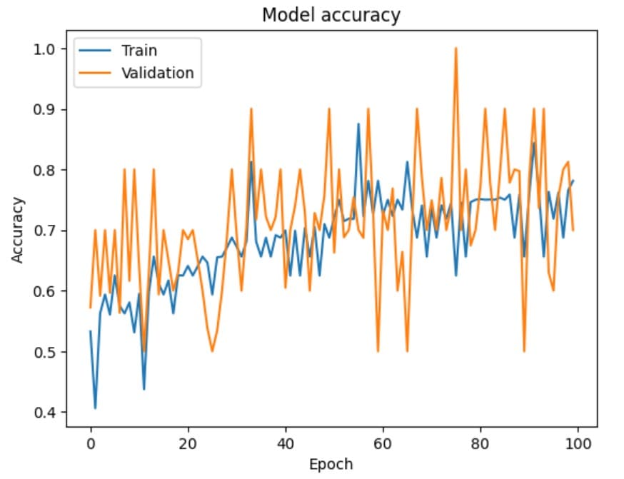
The figure below shows the model’s training accuracy and validation accuracy with respect to the number of epochs. We observe that the accuracy for both the training and validation datasets is increasing with respect to the epoch number.

If the validation accuracy is significantly lower than the training accuracy, it might suggest that the model is overfitting to the training data and not generalizing well to new data. However, this seems to be not a issue for our problem.

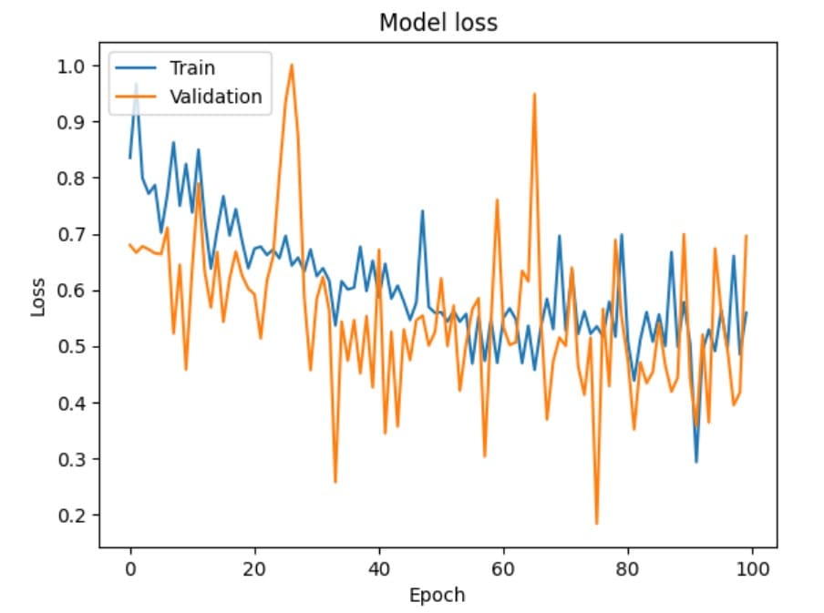
The figure below shows the model’s training loss validation loss with respect to epochs. Both the training and validation loss are decreasing over time and converging which indicates the model is learning and generalizing well to new data.

Conclusions

In this article, we discussed why the birth of AlexNet was a significant leap forward in the field of computer vision. AlexNet showcased the power of deep learning in the 2012 ImageNet challenge and subsequently inspired advancements in neural network design and application.

We further explained the implementation details of the AlexNet model to classify the images of cats and dogs stepwise using Keras and TensorFlow. This guide will give you a practical understanding of building, training, and evaluating a convolutional neural network based on the pioneering AlexNet architecture.

We also highly recommend you evaluate the model performance while varying the hyperparameters such as learning rate, batch size, and number of epochs.

We hope this article is informative and engaging for you. We encourage you to explore the world of deep learning, experiment with different models and datasets, and stay updated on the latest research in this rapidly evolving field. Happy coding and deep learning!

References

Frequently Asked Questions

paravisionlab.co.in

Dr. Partha Majumder is a distinguished researcher specializing in deep learning, artificial intelligence, and AI-driven groundwater modeling. With a prolific track record, his work has been featured in numerous prestigious international journals and conferences. Detailed information about his research can be found on his ResearchGate profile. In addition to his academic achievements, Dr. Majumder is the founder of Paravision Lab, a pioneering startup at the forefront of AI innovation.